Effect of Parallel Environments and Rollout Steps in PPO

This blog post explores batch size in PPO-what happens when we increase the number of parallel environments versus the number of rollout steps, while keeping the total samples per update fixed. We discuss how this affects bias and variance in gradient estimation.

Introduction

In this post, we are going to explore a common dilemma we face when tuning PPO hyperparameters: constructing the batch size.

It’s easy to think of batch size as just a single number, but in PPO, it is actually the product of two distinct levers we can pull:

• The number of parallel environments ($N$).
• The number of steps collected per environment ($T$).

Does it matter if we reach a batch size of 2,048 by running 2 environments for 1,024 steps, or by running 1,024 environments for 2 steps?

Recent work has shown that data collection strategy is not a trivial detail. Multiple studies—including and —highlight that how we distribute experience across environments and rollout lengths can meaningfully influence the stability and effectiveness of on-policy RL methods like PPO. As simulation becomes faster and large-scale parallelism more accessible, understanding these choices is becoming increasingly important.

In this post, we’ll dig into why the structure of the batch matters at all. In particular, we’ll look at how increasing $N$ and increasing $T$ affect the bias and variance of PPO’s gradient estimates, theoretically and empirically. Code for the analysis is provided here

Clarifying Terminology: Batch vs. Mini-Batch

When reading PPO implementations across different libraries, you may notice that the term batch size is used in slightly different ways. To keep things consistent in this post, we’ll use the following terminology as is used in the original PPO paper :

• Rollout Buffer (Total Batch Size): The full dataset collected before a policy update. It is the product of the number of parallel environments ($N$) and the number of steps collected per environment ($T$).

\[\text{Total Batch Size} = N \times T\]

• Mini-Batch: A subset of the Rollout Buffer used for a single gradient descent step. The Rollout Buffer is shuffled and divided into these smaller chunks during training.

Source of Confusion. Different RL libraries sometimes use the word batch to refer to what we’re calling a mini-batch. For example, Stable Baselines3 , Dopamine , OpenAI Baselines (PPO1) , and Ray RLlib commonly adopt this convention. This can lead to ambiguity, especially when tuning PPO’s data collection parameters.

As noted by :

Some common mis-implementations include (1) always using the whole batch for the update, and (2) implementing mini-batches by randomly fetching from the training data, which does not guarantee all training data points are fetched.

Being precise about terminology makes it clear that when we adjust hyperparameters like $N$ and $T$, we’re modifying the amount of experience collected instead of just changing how much data goes into each optimization step (which is determined by the size of each mini-batch).

Background - PPO Gradient Computation

Before diving into bias and variance, let’s write down the gradient PPO computes during policy updates. Ignoring value and entropy terms, the per-sample PPO objective is:

\[L_t^{\text{PPO}}(\theta) = -\min\left(r_t(\theta) \hat{A}_t, \text{clip}(r_t(\theta), 1-\varepsilon, 1+\varepsilon) \hat{A}_t\right),\]

with probability ratio:

\[r_t(\theta) = \frac{\pi_\theta(a_t \mid s_t)}{\pi_{\theta_{\text{old}}}(a_t \mid s_t)}.\]

During a training epoch, PPO updates the policy using mini-batches sampled from the rollout buffer of size $N \times T$. For a mini-batch $M$, the gradient estimate is:

\[G_{mb} = \frac{1}{|M|} \sum_{t \in M} \nabla_\theta L_t^{\text{PPO}}(\theta).\]

Because PPO performs multiple mini-batch updates per iteration, the policy parameters $\theta$ change between these updates. As a result, later mini-batches observe a policy that differs from the one that generated the data, meaning $r_t(\theta) \neq 1$ for most mini-batches.

Additional Info on Clipping

The clipping term prevents the update from moving too far from the behavior policy that produced the data, improving stability during multiple gradient steps by ensuring the new policy stays sufficiently close to the old one for the importance-sampling ratio $r_\theta(t)$ to remain reliable.

Bias and Variance Due to Batch Size

Note:
In this section, we assume that the gradient is computed using the full batch of collected data. This allows us to isolate and analyze the inherent sources of bias and variance that arise purely from the sampled batch itself.
As mentioned in previous section, PPO uses mini-batch stochastic gradient descent, which introduces additional sources of bias and variance due to sub-sampling. These effects will be discussed in the later section.

▶ Simplified Gradient Equation

If we assume that the gradient is computed using the full batch of collected data, we can isolate and analyze the inherent sources of bias and variance that arise purely from the sampled batch itself. Under this assumption, the gradient estimator takes the same form as the standard (vanilla) policy gradient:

$$ G_B = - \frac{1}{N T} \sum_{(s_t, a_t) \in \mathcal{D}} A^{\theta_{\text{old}}}(s_t, a_t)\, \nabla_\theta \log \pi_\theta(a_t \mid s_t) $$

Here, the policy gradient estimate $G_B$ is simply the average of the per-sample policy-gradient contributions $g_i$.

Although the PPO gradient is ultimately derived from the standard (vanilla) policy gradient in a way that supports mini-batch sampling and multiple gradient updates per iteration, it is helpful to “backtrack’’ from the PPO gradient to this full-batch (vanilla) version for clarity.

The policy $\pi_{\theta_{old}}$ is the one used to collect the data, while $\pi_\theta$ is the policy being updated. For the very first full-batch gradient computation of an iteration, we have $\pi_\theta = \pi_{\theta_{old}}$, which implies that the probability ratio satisfies $r = 1$. Because of this, the clipping term does not affect the gradient at this stage. The PPO loss therefore reduces to:

\[L = -\frac{1}{N T} \sum_{(s_t, a_t) \in \mathcal{D}} \underbrace{\frac{\pi_\theta(a_t \mid s_t)}{\pi_{\theta_{\text{old}}}(a_t \mid s_t)}}_{r} \, A^{\theta_{\text{old}}}(s_t, a_t)\]

Taking the gradient of this loss yields:

\[G_B = \nabla_\theta L = -\frac{1}{N T} \sum_{(s_t, a_t) \in \mathcal{D}} \nabla_\theta \left[ r \cdot A^{\theta_{\text{old}}}(s_t, a_t) \right]\]

Since the advantage $A$ is constant with respect to the new policy $\theta$, and knowing that $\nabla_\theta r = r \cdot \nabla_\theta \log \pi_\theta(a_t \mid s_t)$, the gradient simplifies to:

\[\nabla_\theta L = -\frac{1}{N T} \sum_{(s_t, a_t) \in \mathcal{D}} r \, A^{\theta_{\text{old}}}(s_t, a_t) \, \nabla_\theta \log \pi_\theta(a_t \mid s_t)\]

Since $r=1$ in the full-batch case, the equation becomes:

\[G_B = - \frac{1}{N T} \sum_{(s_t, a_t) \in \mathcal{D}} \underbrace{ A^{\theta_{\text{old}}}(s_t, a_t) \, \nabla_\theta \log \pi_\theta(a_t \mid s_t) }_{g_i}\]

▶ Sources of Noise in Gradient Estimation

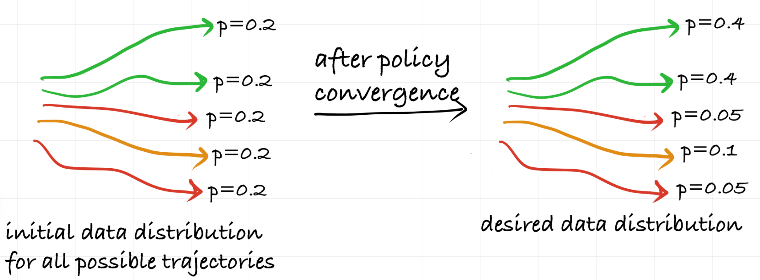
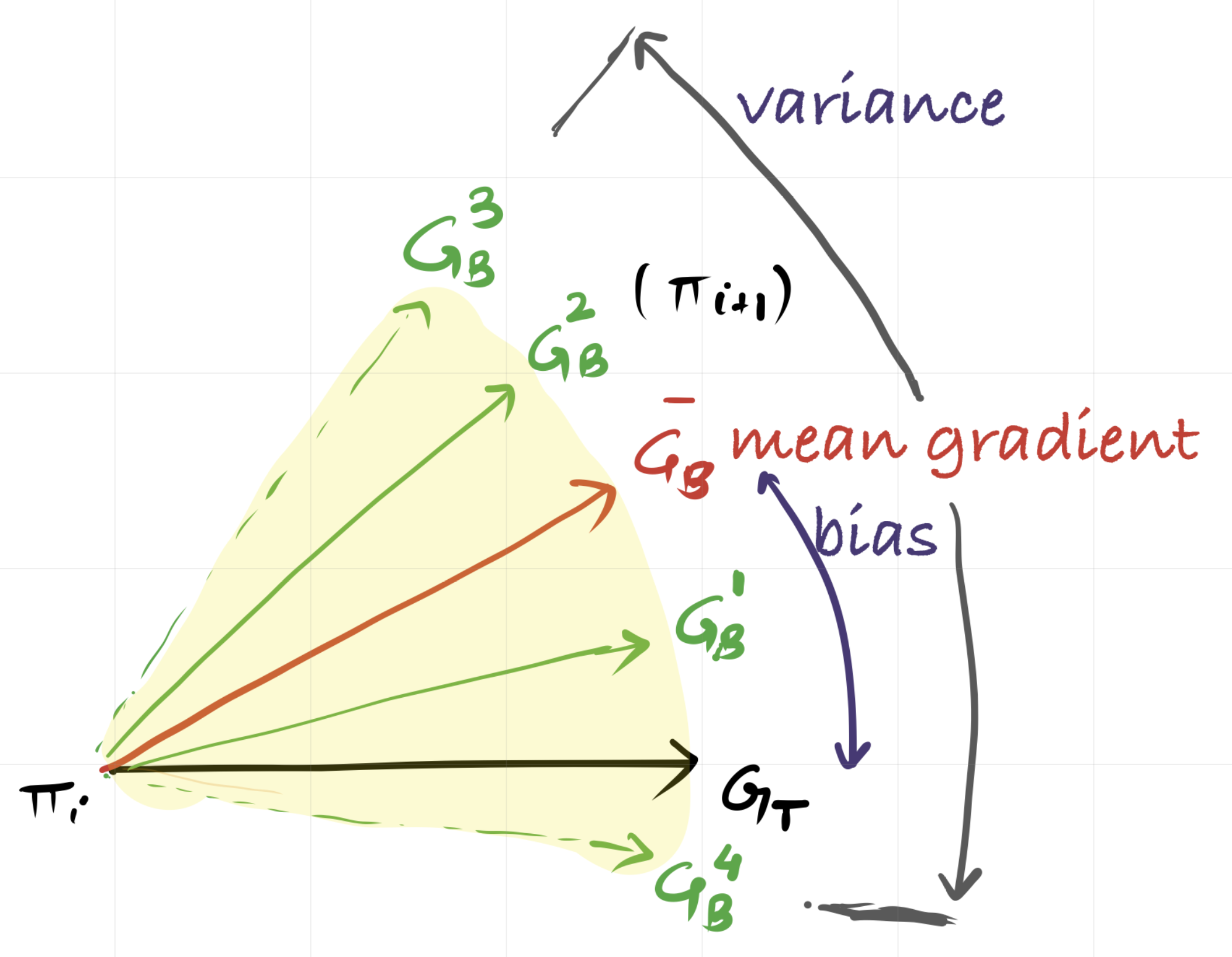
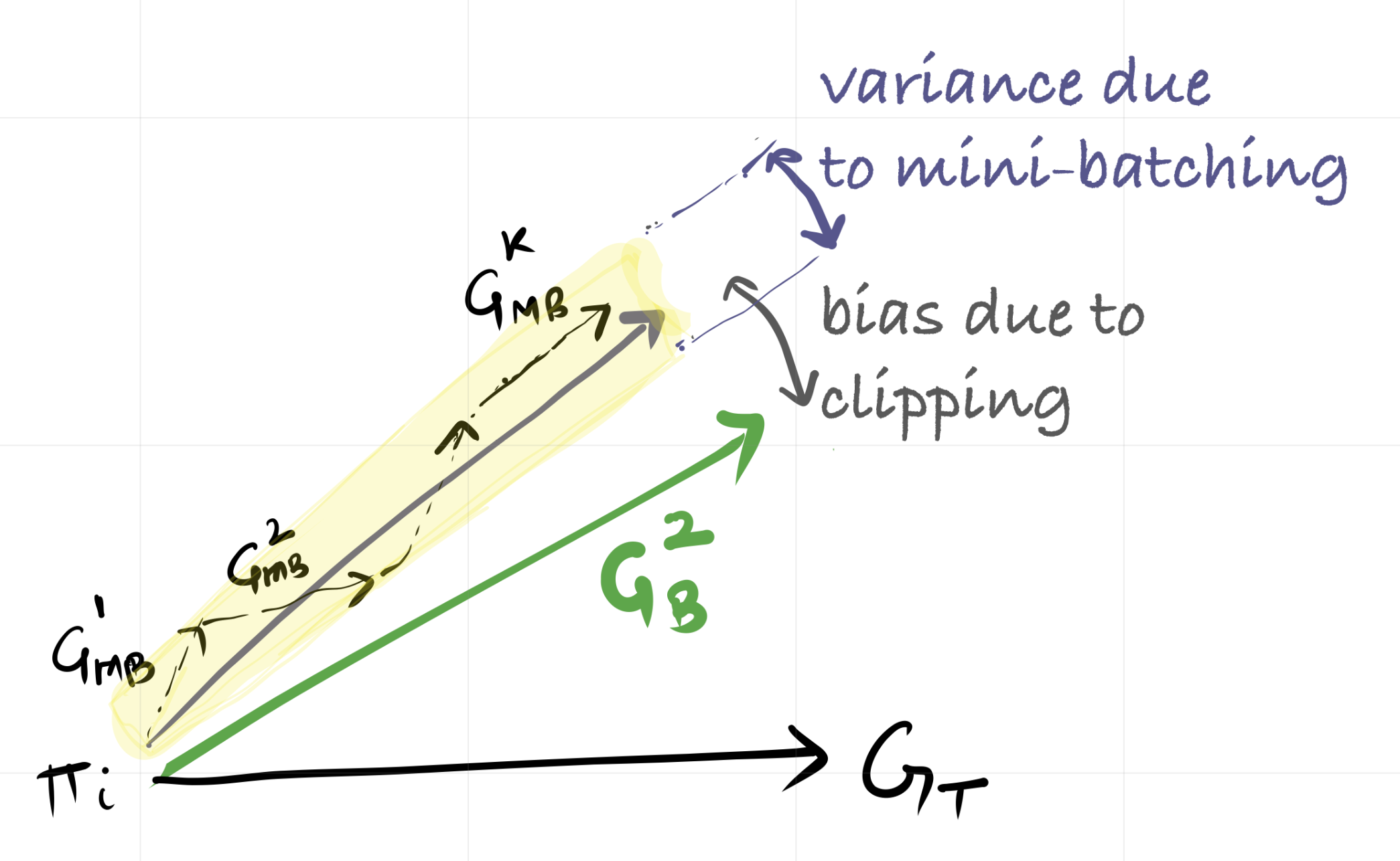
Let us define $G_T$ as the ideal gradient we would obtain with infinite data, or full distribution of trajectories. When PPO estimates a policy gradient, it computes ${G_B}$ from a finite set of sampled trajectories rather than the true gradient $G_T$. This estimator ${G_B}$ is noisy, and it is helpful to describe this noise in terms of two main contributions:

\[G_B \approx G_T + \color{brown}{\text{sampling noise}} + \color{blue}{\text{advantage estimation noise}},\]

where $G_T$ denotes the ideal gradient under the policy’s trajectory distribution.

• The first term, $\color{brown}{\text{sampling noise}}$, is the noise that arises from working with a finite number of samples.
• The second term, $\color{blue}{\text{advantage estimation noise}}$, appears because each gradient $g_i$ is scaled by an advantage estimate $A^{\theta_{\text{old}}}(s_t, a_t)$, which itself is noisy. Since advantage estimation depends on multi-step returns and bootstrapping, two noise sources arise:
  • $\color{blue}{\text{Trajectory Variability Noise}}$ comes from randomness in environment transitions and policy stochasticity. Even small random differences early in a trajectory can lead to large differences in later outcomes and returns.
  • $\color{blue}{\text{Credit Assignment Noise}}$ reflects how difficult it is to determine which early actions contributed to rewards that appear much later. This makes advantage estimates inherently noisy, especially in sparse or delayed reward environments.

Overall, these noise sources appear in the gradient estimator in two ways:

• Variance: how much ${G_B}$ would fluctuate if we collected a different batch from the same policy.
• Bias: the systematic deviation between the expected estimate $\mathbb{E}[{G_B}]$ and the true gradient.

Figure Policy Update: Updating a policy alters the trajectory distribution. A policy update from iteration i to i+1 shifts the probability mass over state–action trajectories, which is what the gradient aims to achieve.

Figure Bias and variance: The estimated gradient Ĝ differs from the true gradient G_T due to sampling variability (variance) and systematic estimation error (bias). Both influence how the policy moves from iteration i to i+1.

▶ Effect of Batch Size on Variance

The variance of the mean gradient is important because it tells us how noisy the update $G_B$ is. A high variance in $G_B$ means that it is an unreliable estimate of the true gradient. Since gradients are vectors, this variance is described by the covariance matrix as follows:

\[\mathrm{Cov}(G_B) = \mathrm{Cov}\left( \frac{1}{NT} \sum_i \bar{g}_i \right)\]

Expanding the covariance of the mean gives

\[\mathrm{Cov}(G_B) = \frac{1}{(NT)^2} \sum_i \mathrm{Cov}(\bar{g}_i) + \frac{1}{(NT)^2} \sum_{i \ne j} \mathrm{Cov}(\bar{g}_i, \bar{g}_j).\]

Because the covariance matrix is high-dimensional, we use its trace as a scalar measure of the noise in the estimate, following . Other scalarizations, such as the Frobenius norm, can be used . Taking the trace of the covariance expression yields the scalar variance:

\[\mathrm{Var}(G_B) = \mathrm{Tr}\big(\mathrm{Cov}(G_B)\big) = \color{blue}{ \underbrace{ \frac{1}{(NT)^2} \sum_i \mathrm{Tr}\big(\mathrm{Cov}(\bar{g}_i)\big) }_{\text{Term 1: Individual Variance}} } + \color{brown}{ \underbrace{ \frac{1}{(NT)^2} \sum_{i \ne j} \mathrm{Tr}\big(\mathrm{Cov}(\bar{g}_i,\bar{g}_j)\big) }_{\text{Term 2: Covariance (Temporal Correlation)}} }.\]

This decomposition connects directly to the noise sources discussed earlier and holds the key to the $N$ vs. $T$ trade-off:

• $\color{blue}{\text{Term 1: Individual Variance}}$

  This term reflects the variability of individual gradient contributions. In practice, this variability arises from both the stochastic policy $\pi_\theta(a_t \mid s_t)$ as well as noise in the advantage estimates, since each $g_i$ is scaled by a noisy advantage value. Importantly, higher individual variance does not necessarily translate into higher variance of the batch-averaged gradient, as gradient cancellation effects and covariance between samples also play a crucial role.

• $\color{brown}{\text{Term 2: Covariance (Temporal Correlation Term)}}$

  This term captures the dependence between gradient samples. Since states within a single episode are temporally correlated, gradients computed from those states are not independent. As a result, the covariance $\mathrm{Cov}(\bar{g}_i,\bar{g}_j)$ need not be zero, and therefore the corresponding scalar term $\mathrm{Tr}\big(\mathrm{Cov}(\bar{g}_i,\bar{g}_j)\big)$ can contribute to the variance.

Impact:
When $T$ is large, the batch contains many highly correlated steps, leading to either large positive or large negative covariance term. This effectively reduces the effective sample size of the batch. This $\color{brown}{\text{increases the sampling noise}}$ because the effective sample size has been reduced. Therefore, a long horizon $T$ can keep $\mathrm{Var}(G_B)$ high. In addition, when $T$ is large, the $\color{blue}{\text{individual variance term also increases}}$, since advantage estimation has high variance over long horizons. (The role of $\lambda$ in GAE will be discussed later.)

When $T$ is small, advantage estimates have lower variance, and the effective sample size is less severely reduced than in the long-horizon case, since fewer temporally correlated states are included. Consequently, the overall variance of the gradient estimator is much lower.

Take-away:
To aggressively reduce variance, we must minimize the covariance term. This requires breaking temporal correlations, which means collecting more independent trajectories—that is, increasing the number of parallel environments, $\mathbf{N}$.

Some Pendulum-v1 Environment Experiments:
To investigate whether policy gradients are correlated along a trajectory, we use the Pendulum-v1 gym environment. PPO is trained with num_envs = 4 and num_steps = 256, which produces a total batch size of batch_size = 4 × 256 = 1024 samples per update.

In the pendulum environment, episodes do not terminate due to task completion or failure; instead, they are truncated after a fixed horizon of 200 time steps . Consequently, all trajectories have a fixed length of 200 steps.

We measure correlation between gradients using the cosine correlation

\[\mathbb{E}\!\left[ \frac{(g_i-\bar g)^\top (g_j-\bar g)} {\|g_i-\bar g\| \, \|g_j-\bar g\|} \right],\]

where $\bar g$ is the mean gradient within the batch. This definition measures directional similarity between two gradients.

Note: relation to covariance-based correlation

Covariance-based correlation A standard covariance-based correlation between two gradients is $$ \frac{ \mathbb{E}\big[(g_i-\mu)^\top (g_j-\mu)\big] }{ \mathbb{E}\|g-\mu\|^2 }. $$ When $g_i$ and $g_j$ come from the same trajectory with lag $k$, this corresponds to the usual lag-$k$ autocorrelation used in time-series analysis and effective sample size estimation. Using the definition above, we compute the correlation between gradients at different lags and plot the result below. The plotted curve is averaged over 20 training checkpoints, and the shaded region shows variability across checkpoints. 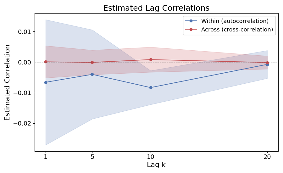The covariance-based correlation is close to zero for all lags, although within-trajectory estimates show larger variation at small lags and approach the across-trajectory baseline as the lag increases. This suggests short-range dependence, but covariance-based correlation averages signed inner products, so positive and negative alignments can cancel in high-dimensional gradients. We therefore use the cosine correlation above, which normalizes each pair individually and better captures directional alignment between gradients.

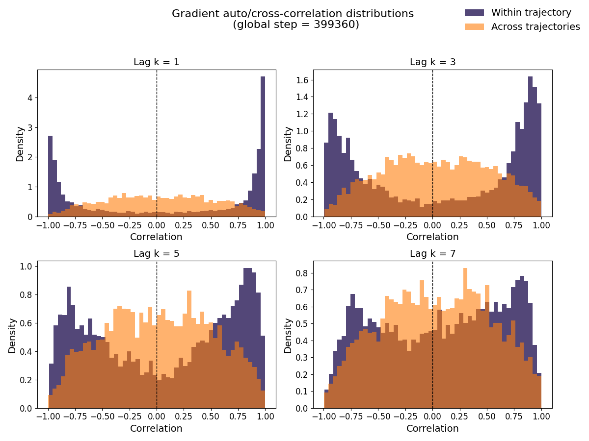
At a certain training update, we analyze gradient correlation at two levels: For a particular step in training, we compute following:

• Within-trajectory correlation: correlation between gradients $g_t$ and $g_{t+k}$ sampled from the same trajectory at temporal lag $k$.
• Across-trajectory correlation: correlation between gradients sampled from two different trajectories, each selected at random. For within trajectory correlation we test it for different values of lag k.

Gradients within the same trajectory are expected to be more strongly correlated, while gradients sampled across trajectories provide a baseline that serves as approximately independent samples.

The below figure compares the correlation of gradients within a trajectory to that of gradients across different trajectories at two different points during training.

Figure: Comparison of within-trajectory and across-trajectory gradient correlation at global step 399360 for lag values \(k = 1, 3, 5, 7\).

Figure: Comparison of within-trajectory and across-trajectory gradient correlation at global step 450560 for lag values \(k = 1, 5, 10, 40\).

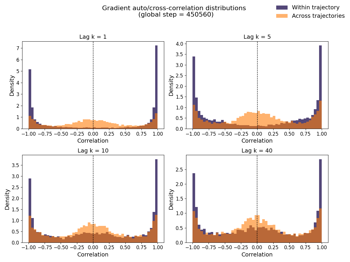
The higher correlation observed within trajectories suggests that num_steps can influence the diversity of gradient directions within a batch. To study this effect more systematically, let us analyze two settings: num_envs = 4, num_steps = 256 (long trajectories) and num_envs = 16, num_steps = 64 (short trajectories). Let us focus on training step 450560 now, as the correlation effects remain visible even at large lags (i.e. $k$=40).

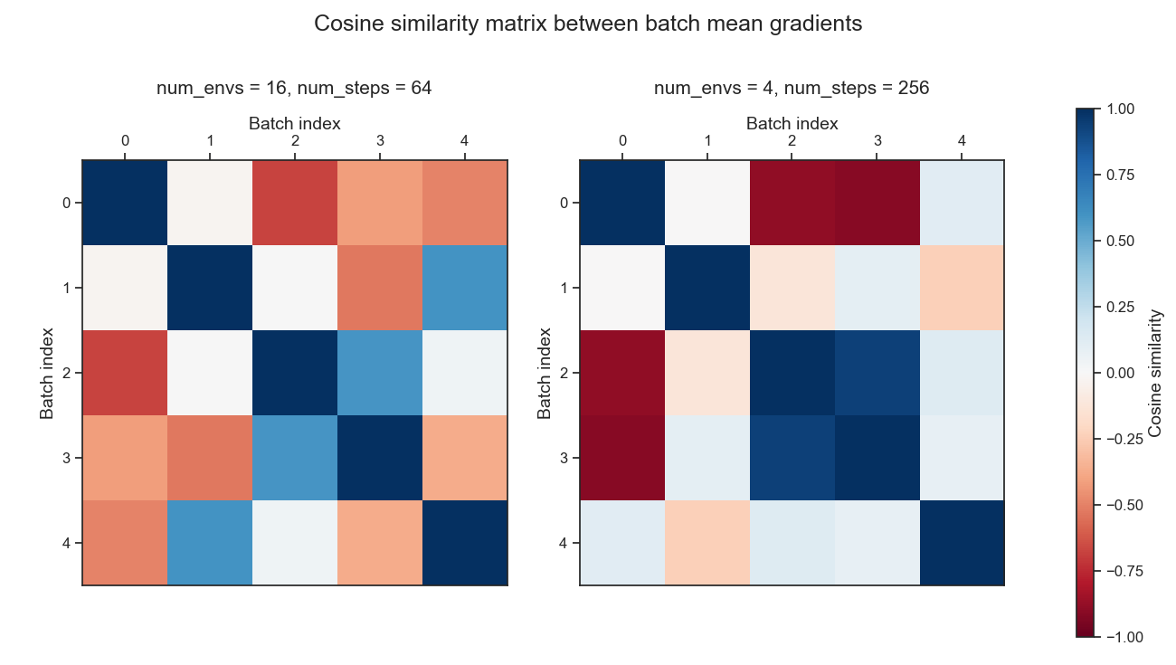
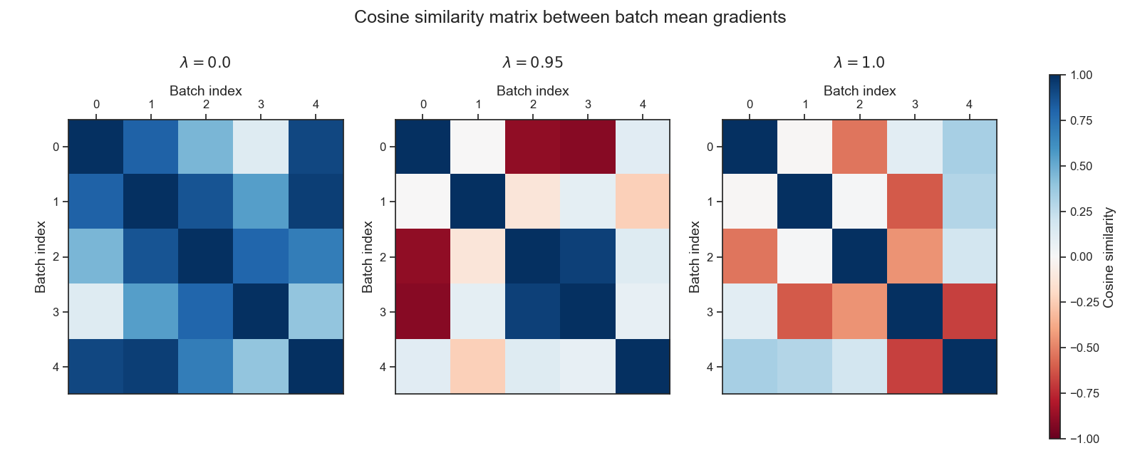
For each setting, we randomly sample five batches from the rollout buffer (batch0 … batch4). From each batch, we compute the mean gradient vector, and then compute pairwise cosine similarities:

\[\cos(\bar{g}^{(i)}, \bar{g}^{(j)}) = \frac{\bar{g}^{(i)} \cdot \bar{g}^{(j)}}{\lVert \bar{g}^{(i)} \rVert \, \lVert \bar{g}^{(j)} \rVert }.\]

This allows us to visualize whether the mean gradient from one batch tends to point in the same direction as the mean gradient from another batch.

Importantly, the differences we observe between batches represent the overall variance of the gradient estimator. This includes both the per-sample variance (noise in each $(g_i)$) and the additional covariance created by temporal correlations within trajectories.

In the long-horizon case (4×256), the off-diagonal cells of the cosine similarity heatmap shows that mean gradients from different batches can be strongly positively or negatively correlated. Negative correlation indicates that the gradient estimate from one batch points in the opposite direction of another batch’s mean gradient, revealing substantial variance in the gradient estimator. In contrast, in the short-horizon case (16x64), while negatively correlated batch mean gradients do occur, they are noticeably less severe than in the long-horizon setting, indicating reduced gradient variance.

Figure: Cosine similarity between batch mean gradients for short-horizon and long-horizon settings. The long-horizon case (4×256) on the right exhibits stronger positive and negative off-diagonal correlations, suggesting increased variability in gradient estimates.

▶ Effect of Batch Size on Bias

Bias describes consistent displacement between the estimated gradient and the true gradient:

\[\text{Bias} = \mathbb{E}[{G_B}] - G_T.\]

In PPO, bias arises mainly through how returns or advantages are estimated. Generalized Advantage Estimation rely on bootstrapping via Value function estimates, and can introduce bias if the value function is inaccurate, but provides lower variance.

The effect of the rollout length $T$ on bias is as follows:

• When $T$ is small, advantage estimates rely more heavily on bootstrapping, which increases bias. This shows up in practice as noisier advantage estimates.

• When $T$ is large, advantage estimates use more actual returns and rely less on the value function, so bias becomes smaller.

Importantly, correlation between samples (the covariance term) affects variance but does not affect bias as it is determined by how advantages are computed.

Bias and Variance Due to Mini-batches

Mini-batches are used because the rollout buffer is typically large, and multiple updates per iteration improve computational efficiency. However, mini-batching also introduces sub-sampling variance, since each mini-batch represents only a portion of the available data. Clipped objectives modify the effective update direction, and introduce another form of bias in the gradient estimate.

Figure: Mini-batch gradients: Mini-batch updates compute gradient estimates from subsets of the full batch. These estimates vary across mini-batches and accumulate over an update epoch, introducing sub-sampling variance and policy drift related bias.

What role does GAE-$\lambda$ play here?

\[A^{\text{GAE}}(\gamma, \lambda)_t = \sum_{l=0}^{\infty} (\gamma \lambda)^l \delta_{t+l}\]

where $\delta_t = r_t + \gamma V(s_{t+1}) - V(s_t)$ and corresponds to the one-step temporal-difference error.

For $\lambda = 0$, this reduces to \(A^{\text{GAE}}(\gamma, 0)_t = \delta_t = r_t + \gamma V(s_{t+1}) - V(s_t)\) which only considers immediate rewards and bootstrapped values. This has low variance (the environment stochasiticity only affects a single step) but can be biased due to the bootstrapping from the value function, which is still being learned.

For $\lambda = 1$, it becomes the Monte Carlo return: \(A^{\text{GAE}}(\gamma, 1)_t = \sum_{l=0}^{\infty} \gamma^l \delta_{t+l} = \sum_{l=0}^{\infty} \gamma^l r_{t+l} - V(s_t)\) which incorporates the full sequence of rewards until the end of the episode. This is a accurate (unbiased) estimate of the advantage, as it is based on actual observed returns, opposed to boostrapped values from value estimates. However, it has high variance because the returns can be highly variable, especially in stochastic and sensitive environments.

$\lambda$ thus controls how much we rely on immediate rewards vs long-term returns. Now, the advantages are computed for the collected batch of size $NT$, and “how far into the future” is limited by $T$, the rollout steps. When $T$ is much smaller than the episode length (especially for recurrent environments ), the advantage estimates will be truncated, effectively creating the same effect as a lower $\lambda$. For $T > $ episode length, the advantage estimates is unaffected.

Based on this reasoning, one might expect the impact of $\lambda$ on gradient variance to depend strongly on the rollout horizon $T$. However, empirical results do not show a clean separation between short-horizon and long-horizon settings. Instead, varying $\lambda$ produces qualitatively similar effects across both regimes.

In particular, changing $\lambda$ does not eliminate temporal correlation between gradients sampled along a trajectory. Even for $\lambda = 0$, gradients remain correlated across time due to shared state visitation and common policy. What $\lambda$ primarily influences is directional coherence: as $\lambda$ increases, per-sample gradient directions become more variable, which weakens alignment within a batch.

Figure: Within-trajectory and across-trajectory correlation for the 4×256 setup. Even for $\lambda = 0$ and $\lambda = 1$, gradients remain correlated at large temporal lags (here, $k = 40$).

Figure: Cosine similarity between each per-sample gradient and the batch mean gradient, computed as $ \cos(g_i, \bar{g}^{(i)}) = \frac{g_i \cdot \bar{g}^{(i)}}{\lVert g_i \rVert \, \lVert \bar{g}^{(i)} \rVert}. $ As $\lambda$ increases, the distribution becomes more concentrated around zero, indicating increased variability in per-sample gradient directions.

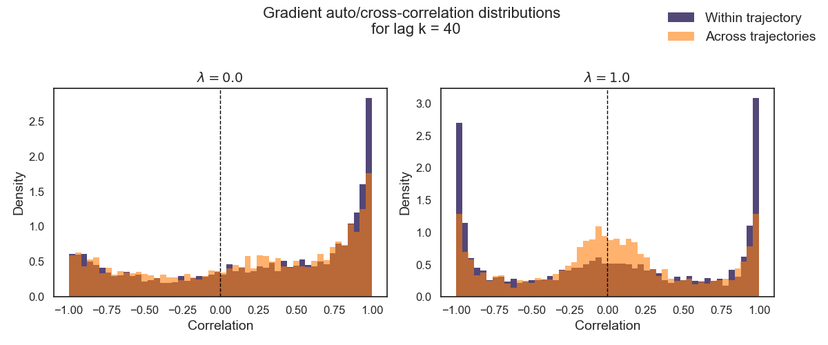
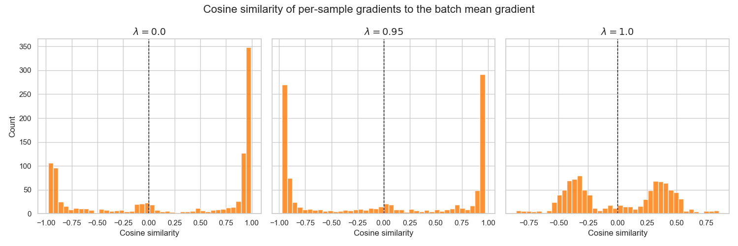
Varying the GAE parameter $\lambda$ therefore primarily affects the directional variability of per-sample gradients within a batch rather than removing temporal correlation altogether. For larger values of $\lambda$, gradients tend to point in more diverse directions, leading to partial cancellation when averaged. As a result, batch mean gradients may appear less extreme and, in some cases, more consistently aligned across batches.

For smaller values of $\lambda$, per-sample gradients are often more directionally consistent within a batch. This can produce strongly aligned batch mean gradients, which may result in either low or high batch-to-batch variance depending on the rollout and trajectory correlations.

Figure: Pairwise cosine similarity between batch mean gradients. For $\lambda = 0$, batch-to-batch variance can be either low or high depending on the rollout. For larger $\lambda$, cancellation within batches can reduce extreme batch-to-batch variance.

Wrapping-up

This post examined how the rollout length $T$ and the number of parallel environments $N$ affects the variance of gradient estimates. Longer rollouts introduce strong temporal correlations between gradients computed from neighboring time steps, which can substantially increase variance despite a fixed total batch size. Increasing the number of parallel environments instead reduces these correlations by collecting more independent trajectories.

In practice, PPO implementations further mitigate correlation effects by shuffling the rollout buffer and performing updates using mini-batches. This randomization breaks up temporally adjacent samples and partially reduces gradient correlation. Nevertheless, the choice of $N$ and $T$ directly influences the stability of the learning dynamics.