A Hitchhiker's Guide to Momentum

Polyak momentum is one of the most iconic methods in optimization. Despite it's simplicity, it features rich dynamics that depend both on the step-size and momentum parameter. In this blog post we identify the different regions of the parameter space and discuss their convergence properties using the theory of Chebyshev polynomials.

Dedicated to the memory of Boris Polyak (May 4, 1935 - February 3, 2023), inventor of this method and pioneer of the field of optimization.

Gradient Descent with Momentum

Gradient descent with momentum, also known as heavy ball or momentum for short, is an optimization method designed to solve unconstrained minimization problems of the form \begin{equation} \argmin_{\xx \in \RR^d} \, f(\xx)\,, \end{equation} where the objective function $f$ is differentiable and we have access to its gradient $\nabla f$. In this method the update is a sum of two terms. The first term is the difference between the current and the previous iterate $(\xx_{t} - \xx_{t-1})$, also known as momentum term. The second term is the gradient $\nabla f(\xx_t)$ of the objective function.

Gradient Descent with Momentum
Input: starting guess $\xx_0$, step-size $\step > 0$ and momentum parameter $\mom \in (0, 1)$.
$\xx_1 = \xx_0 - \dfrac{\step}{\mom+1} \nabla f(\xx_0)$
For $t=1, 2, \ldots$ compute \begin{equation}\label{eq:momentum_update} \xx_{t+1} = \xx_t + \mom(\xx_{t} - \xx_{t-1}) - \step\nabla f(\xx_t) \end{equation}

Despite its simplicity, gradient descent with momentum exhibits unexpectedly rich dynamics that we’ll explore on this post.

History and relatex work

The origins of momentum can be traced back to Frankel’s method in the 1950s for solving linear system of equations. It was later generalized by Boris Polyak to non-quadratic objectives. While the quadratic case is by now well understood, the general strongly convex case has instead had some fascinating developments in the last years. In the convex (but not strongly convex) case, Ghadimi et al. showed the global convergence of the method in 2015. One year later, Lessard, Recht and Packard surprised the community with an example of a on-dimensional Lipschitz gradient and strongly convex function where the heavy-ball method (with a specific choice of parameters) doesn’t converge nor diverge, but cycles instead.

A paper that also explores the dynamics of momentum is Gabriel Goh’s excellent Why Momentum Really Works. There are subtle but important differences between both analysis. The landscape described in the section “The Dynamics of Momentum” describe the improvement along the direction of a single eigenvector. This partial view produces some misleading conclusions. For example, along the direction of a single eigenvector, the largest improvement is achieved with zero momentum and a step-size of 1 over the associated eigenvalue. This conclusion however doesn’t hold in higher dimensions, where as we will see, the momentum term that yields the fastest convergence is non-zero.

A stochastic variant of this method, where the gradient is replaced by a stochastic estimate, is one of the most popular methods for deep learning. This has led in recent years to a flurry of research –and improved understanding – of this stochastic variant. Although we won’t be analyzing the stochastic variant, due to its importance, let us briefly mention some recent works.

One of the first works to highlight the importance of momentum for training deep neural networks is the 2013 paper by Sutskever et al. Some recent progress in the field has been possible by viewing the stochastic variant as an averaging method. This has led to the development of improved last-iterate convergence rates and a better understanding of it’s behavior in the non-convex setting. Another fruitful line of work has been to consider the overparametrized (or interpolation) setting, where the variance of the updates vanishes at the optimum. In this regime, different momentum-like methods have been shown to enjoy a faster worst-case convergence rate than SGD.

How Fast is Momentum?

Momentum is fast. So fast that it’s often the default choice of machine learning practitioners. But can we quantify this more precisely?

Throughout the post we’ll assume that our objective function $f$ is a quadratic objective of the form \begin{equation}\label{eq:opt} f(\xx) \defas \frac{1}{2}(\xx - \xx^\star) \HH (\xx - \xx^\star)~, \end{equation} where $\HH$ is a symmetric positive definite matrix and $\xx^\star$ is the minimizer of the objective. We’ll assume that the eigenvalues of $\HH$ are in the interval $[\mu, L]$, where $\mu$ is strictly positive by the PSD assumption.

The measure we’ll use to quantify the speed of convergence is the rate of convergence. This is the worst-case relative improvement in the iterate suboptimality at iteration $t$, defined as \begin{equation}\label{eq:convergence_rate} r_t \defas \sup_{\xx_0, \text{eigs}(\HH) \in [\mu, L]} \frac{\|\xx_{t} - \xx^\star\|}{\|\xx_{0} - \xx^\star\|}\,. \end{equation} This is a worst-case measure because of all problem instances, we take worst possible initialization $\xx_0$ and matrix $\HH$ with eigenvalues in the interval $[\mu, L]$.

This is a measure of how much progress is made (in the worst-case) at iteration $t$. The smaller the value of $r_t$, the faster the algorithm converges. Since all algorithms that we consider converge exponentially fast, for large enough $t$ the error is of the order of $\mathcal{O}{(\text{constant}^t)}$. Hence the most informative quantity is the value of $\text{constant}$ in this expression. We’ll call this quantity the asymptotic rate of convergence, and denote it: \begin{equation} r_{\infty} \defas \limsup_{t \to \infty} \sqrt[t]{r_t}\,. \end{equation} This is the quantity we’ll be discussing throughout the post and what we’ll use to compare the speed of momentum for different values of its hyperparameters.

A connection between optimization methods and polynomials

To compute easily the asymptotic rate of convergence for all admissible values of step-size and momentum, we’ll use a connection between optimization of quadratic functions and the theory of orthogonal polynomials. This theory was extensively used in the early days of numerical analysis and provides an elegant and simple way to compute asymptotic rates (and non-asymptotic ones, although not the topic of this blog post) from known results in the theory of orthogonal polynomials. We favor this technique for its simplicity and elegance, although ones that also be used with identical results. Other techniques include the linear operator technique used by Polyak, the estimate sequences technique pioneered by Nesterov or the use of Lyapunov functions.

The main result that will allow us to make the link between optimization and orthogonal polynomials is the following result. It’s origins seem unclear, although a proof can be found in the 1959 monograph of Rutishauser.

Consider the following polynomial $P_t$ of degree $t$, defined recursively as: \begin{equation} \begin{split} &P_{t+1}(\lambda) = (1 + \mom - \step \lambda ) P_{t}(\lambda) - \mom P_{t-1}(\lambda)\\ &P_1(\lambda) = 1 - \frac{\step}{1 + \mom} \lambda\,, ~ P_0(\lambda) = 1\,,~ \end{split}\label{eq:def_residual_polynomial2} \end{equation} Then we can write the suboptimality at iteration $t$ as \begin{equation} \xx_t - \xx^\star = P_t(\HH) \left( \xx_0 - \xx^\star \right) \,, \end{equation} where $P_t(\HH)$ is the matrix obtained from evaluating the (originally real-valued) polynomial $P_t$ at the matrix $\HH$.

This last identity will allow us to easily compute convergence rates. In particular, plugging it into the definition of the convergence rate \eqref{eq:convergence_rate} we get that the rate is determined by the absolute value of the residual polynomial over the $[\mu, L]$ interval: \begin{align} r_t &= \sup_{\xx_0, \text{eigs}(\HH) \in [\mu, L]} \frac{\|P_t(\HH) \left( \xx_0 - \xx^\star \right)\|}{\|\xx_{0} - \xx^\star\|} \\ & = \sup_{\text{eigs}(\HH) \in [\mu, L]} \|P_t(\HH)\| \\ & = \sup_{\lambda \in [\mu, L]} \lvert P_t(\lambda) \rvert\,. \end{align} We’ve now reduced the problem of computing the convergence rate to the problem of computing the absolute value of a polynomial over a given interval. This is a problem that has been extensively studied in the theory of orthogonal polynomials. In particular, we’ll use known bounds on Chebyshev polynomials of the first and second kind, as the residual polynomial of momentum can be written as a convex combination of these two polynomials. This fact is proven in the next result, which is a generalization of equation (II.29) in (Rutishauser 1959).

The residual polynomial of momentum can be written in terms of Chebyshev polynomials of the first and second kind as \begin{align} P_t(\lambda) = \mom^{t/2} \left( {\small\frac{2\mom}{1+\mom}}\, T_t(\sigma(\lambda)) + {\small\frac{1 - \mom}{1 + \mom}}\,U_t(\sigma(\lambda))\right)\,. \end{align} where $\sigma(\lambda) = {\small\dfrac{1}{2\sqrt{\mom}}}(1 + \mom - \step\,\lambda)\,$ is a linear function that we'll refer to as the link function and $T_t$ and $U_t$ are the Chebyshev polynomials of the first and second kind respectively.

Show proof

Let's denote by $\widetilde{P}_t$ the right hand side of the above equation, that is, \begin{equation} \widetilde{P}_{t}(\lambda) \defas \mom^{t/2} \left( {\small\frac{2 \mom}{1 + \mom}}\, T_t(\sigma(\lambda)) + {\small\frac{1 - \mom}{1 + \mom}}\, U_t(\sigma(\lambda))\right)\,. \end{equation} Our goal is to show that $P_t = \widetilde{P}_t$ for all $t$.

For $t=1$, $T_1(\lambda) = \lambda$ and $U_1(\lambda) = 2\lambda$, so we have \begin{align} \widetilde{P}_1(\lambda) &= \sqrt{\mom} \left(\tfrac{2 \mom}{1 + \mom} \sigma(\lambda) + \tfrac{1 - \mom}{1 + \mom} 2 \sigma(\lambda)\right)\\ &= \frac{2 \sqrt{\mom}}{1 + \mom} \sigma(\lambda) = 1 - \frac{\step}{1 + \mom} \lambda\,, \end{align} which corresponds to the definition of $P_1$ in \eqref{eq:def_residual_polynomial2}.

Assume it's true for any iteration up to $t$, we will show it's true for $t+1$. Using the three-term recurrence of Chebyshev polynomials we have \begin{align} &\widetilde{P}_{t+1}(\lambda) = \mom^{(t+1)/2} \left( {\small\frac{2 \mom}{1 + \mom}}\, T_{t+1}(\sigma(\lambda)) + {\small\frac{1 - \mom}{1 + \mom}}\, U_{t+1}(\sigma(\lambda))\right) \\ &= \mom^{(t+1)/2} \Big( {\small\frac{2 \mom}{1 + \mom}}\, (2 \sigma(\lambda) T_{t}(\sigma(\lambda)) - T_{t-1}(\sigma(\lambda))) \nonumber\\ &\qquad\qquad + {\small\frac{1 - \mom}{1 + \mom}}\, (2 \sigma(\lambda) U_{t}(\sigma(\lambda)) - U_{t-1}(\sigma(\lambda)))\Big)\\ &= 2 \sigma(\lambda) \sqrt{\mom} P_t(\lambda) - \mom P_{t-1}(\lambda)\\ &= (1 + \mom - \step \lambda) P_t(\lambda) - \mom P_{t-1}(\lambda) \end{align} where the third identity follows from grouping polynomials of same degree and the induction hypothesis. The last expression is the recursive definition of $P_{t+1}$ in \eqref{eq:def_residual_polynomial2}, which proves the desired $\widetilde{P}_{t+1} = {P}_{t+1}$.

Tools of the trade: the two faces of Chebyshev polynomials

A key feature that we’ll use extensively about Chebyshev polynomials is that they behave very differently inside and outside the interval $[-1, 1]$. Inside this interval (shaded blue region) the magnitude of these polynomials stays close to zero, while outside it explodes:

Let’s make this observation more precise.

Inside the $[-1, 1]$ interval, Chebyshev polynomials admit the trigonometric definitions $T_t(\cos(\theta)) = \cos(t \theta)$ and $U_{t}(\cos(\theta)) = \sin((t+1)\theta) / \sin(\theta)$ and so they have an oscillatory behavior with values bounded in absolute value by 1 and $t+1$ respectively.

Outside of this interval the Chebyshev polynomials of the first kind admit the explicit form for $|\xi| \ge 1$: \begin{align} T_t(\xi) &= \dfrac{1}{2} \Big(\xi-\sqrt{\xi^2-1} \Big)^t + \dfrac{1}{2} \Big(\xi+\sqrt{\xi^2-1} \Big)^t \\ U_t(\xi) &= \frac{(\xi + \sqrt{\xi^2 - 1})^{t+1} - (\xi - \sqrt{\xi^2 - 1})^{t+1}}{2 \sqrt{\xi^2 - 1}}\,. \end{align} We’re interested in convergence rates, so we’ll look into $t$-th root asymptotics of the quantities.With little extra effort, it would be possible to derive non-asymptotic convergence rates, although I won't pursue this analysis here. Luckily, these asymptotics are the same for both polynomialsAlthough we won't use it here, this $t$-th root asymptotic holds for (almost) all orthogonal polynomials, not just Chebyshev polynomials. See for instance reference below and taking limits we have that \begin{equation} \lim_{t \to \infty} \sqrt[t]{|T_t(\xi)|} = \lim_{t \to \infty} \sqrt[t]{|U_t(\xi)|} = |\xi| + \sqrt{\xi^2 - 1}\,. \end{equation}

The Robust Region

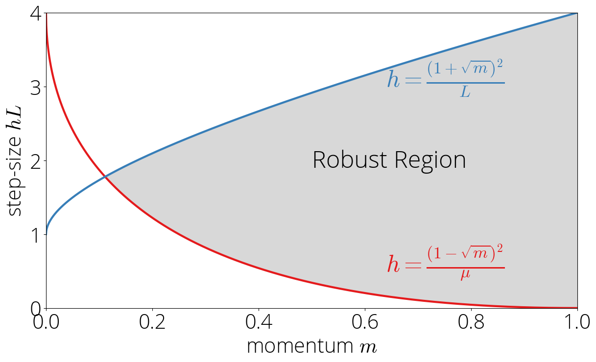
Let’s start first by considering the case in which the image of $\sigma$ is in the $[-1, 1]$ interval. This is the most favorable case. In this case, the Chebyshev polynomials are bounded in absolute value by 1 and $t+1$ respectively. Since the Chebsyshev polynomials are evaluated at $\sigma(\cdot)$, this implies that $\lvert \sigma(\lambda)\rvert \leq 1$. We’ll call the set of step-size and momentum parameters for which the previous inequality is verified the robust region.

Let’s visualize this region in a map. Since $\sigma$ is a linear function, its extremal values are reached at the edges: \begin{equation} \max_{\lambda \in [\lmin, \lmax]} |\sigma(\lambda)| = \max{|\sigma(\lmin)|, |\sigma(\lmax)|}\,. \end{equation} Using $\lmin \leq \lmax$ and that $\sigma(\lambda)$ is decreasing in $\lambda$, we can simplify the condition $\lvert \sigma(\lambda)\rvert \leq 1$ to $\sigma(\lmin) \leq 1$ and $\sigma(L) \geq -1$, which in terms of the step-size and momentum correspond to: \begin{equation}\label{eq:robust_region} \frac{(1 - \sqrt{\mom})^2}{\lmin} \leq \step \leq \frac{(1 + \sqrt{\mom})^2}{L} \,. \end{equation} These two conditions provide the upper and lower bound of the robust region.

Asymptotic rate

Let $\sigma(\lambda) = \cos(\theta)$ for some $\theta$, which is always possible since $\sigma(\lambda) \in [-1, 1]$. In this regime, Chebyshev polynomials verify the identities $T_t(\cos(\theta)) = \cos(t \theta)$ and $U_t(\cos(\theta)) = \sin((t+1)\theta)/\sin(\theta)$ , which replacing in the definition of the residual polynomial gives \begin{equation} P_t(\sigma^{-1}(\cos(\theta))) = \mom^{t/2} \left[ {\small\frac{2\mom}{1+\mom}}\, \cos(t\theta) + {\small\frac{1 - \mom}{1 + \mom}}\,\frac{\sin((t+1)\theta)}{\sin(\theta)}\right]\,. \end{equation}

Since the expression inside the square brackets is bounded in absolute value by $t+2$, taking $t$-th root and then limits we have $\limsup_{t \to \infty} \sqrt[t]{\lvert P_t(\sigma^{-1}(\cos(\theta)))\rvert} = \sqrt{\mom}$ for any $\theta$. This gives our first asymptotic rate:

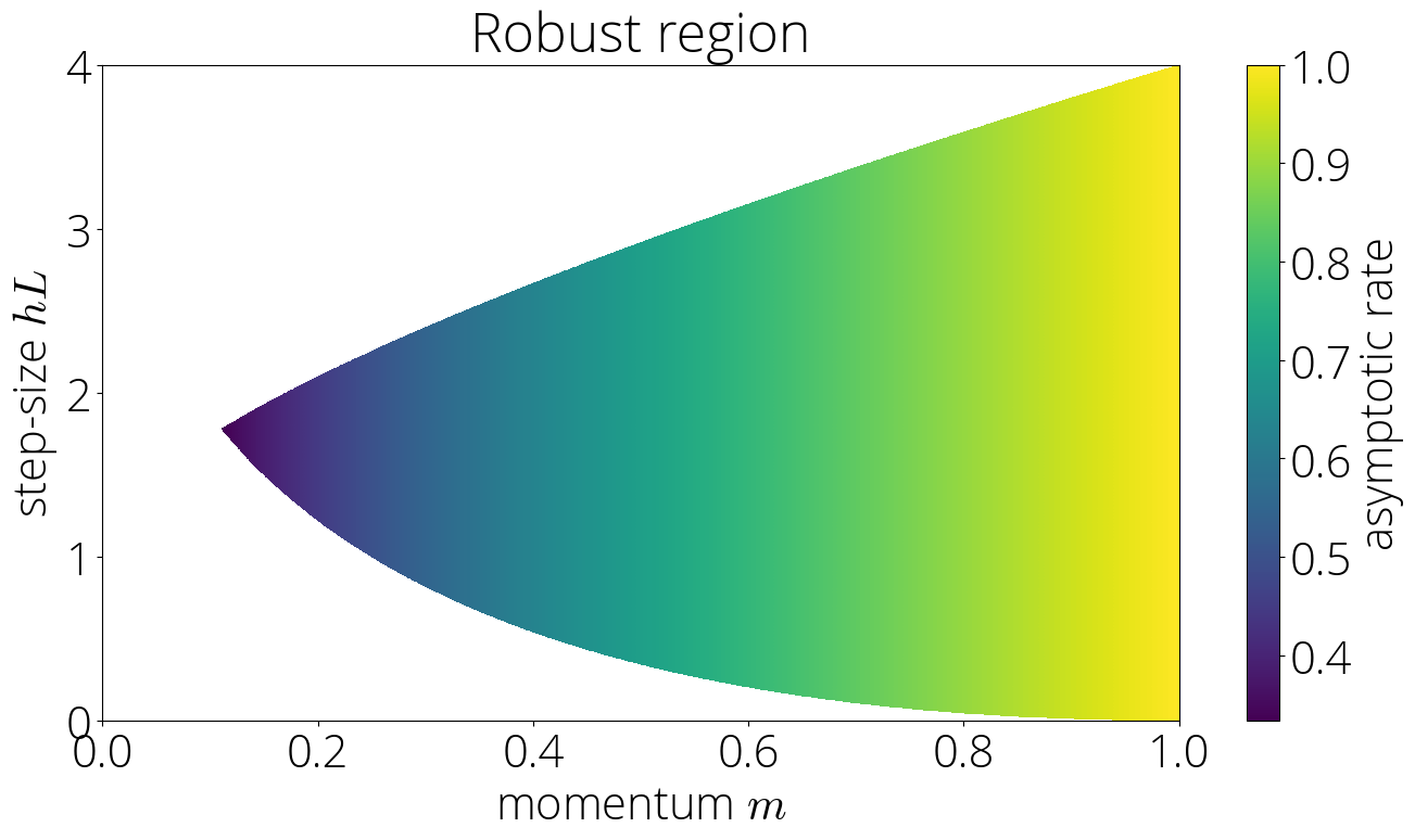
The asymptotic rate in the robust region is $r_{\infty} = \sqrt{\mom}$.

This is nothing short of magical. It would seem natural –and this will be the case in other regions– that the speed of convergence should depend on both the step-size and the momentum parameter. Yet, this result implies that it’s not the case in the robust region. In this region, the convergence only depends on the momentum parameter $\mom$. Amazing.This insensitivity to step-size has been leveraged by Zhang et al. 2018 to develop a momentum tuner

This also illustrates why we call this the robust region. In its interior, perturbing the step-size in a way that we stay within the region has no effect on the convergence rate. The next figure displays the asymptotic rate (darker is faster) in the robust region.

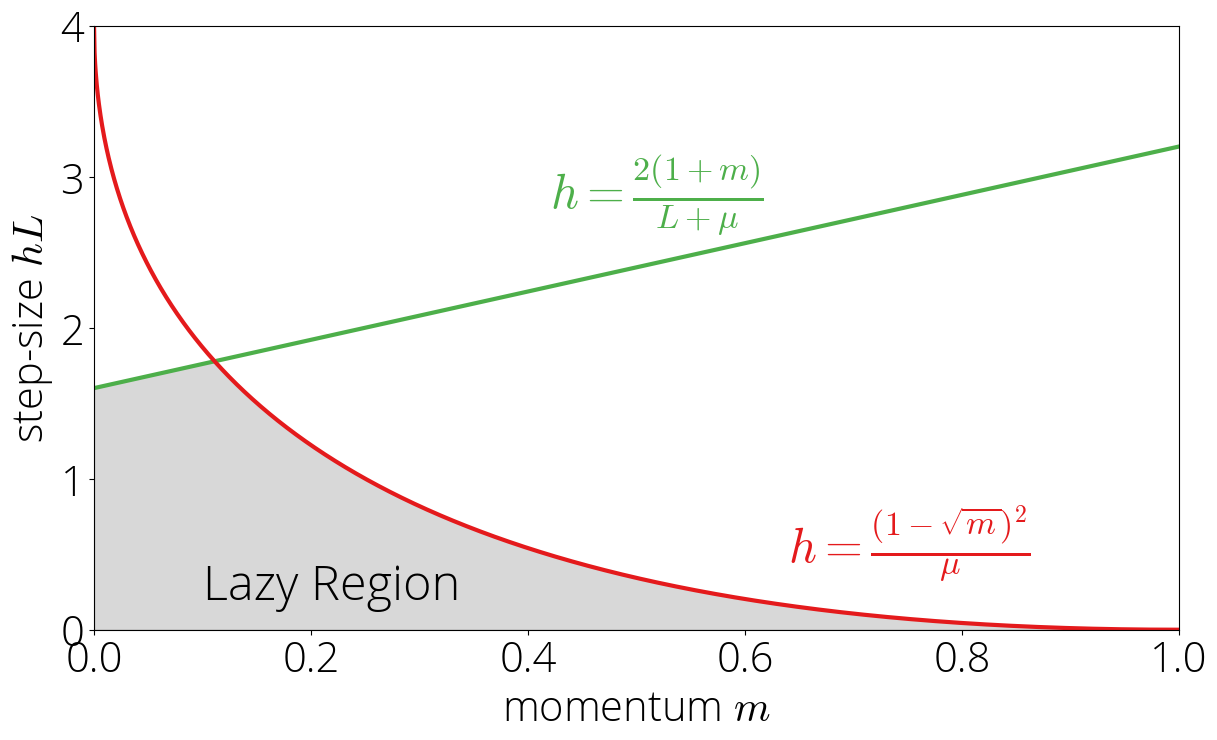
The Lazy Region

Let’s consider now what happens outside of the robust region. In this case, the convergence will depend on the largest of $\{\lvert\sigma(\lmin)\rvert, \lvert\sigma(L)\rvert\}$. We’ll consider first the case in which the maximum is $\lvert\sigma(\lmin)\rvert$ and leave the other one for next section.

This region is determined by the inequalities $\lvert\sigma(\lmin)\rvert > 1$ and $\lvert\sigma(\lmin)\rvert \geq \lvert\sigma(L)\rvert$. Using the definition of $\sigma$ and solving for $\step$ gives the equivalent conditions \begin{equation} \step \leq \frac{2(1 + \mom)}{L + \lmin} \quad \text{ and }\quad \step \leq \frac{(1 - \sqrt{\mom})^2}{\lmin}\,. \end{equation} Note the second inequality is the same one as for the robust region \eqref{eq:robust_region} but with the inequality sign reversed, and so the region will be on the oposite side of that curve. We’ll call this the lazy region, as in increasing the momentum will take us out of it and into the robust region.

Asymptotic rate

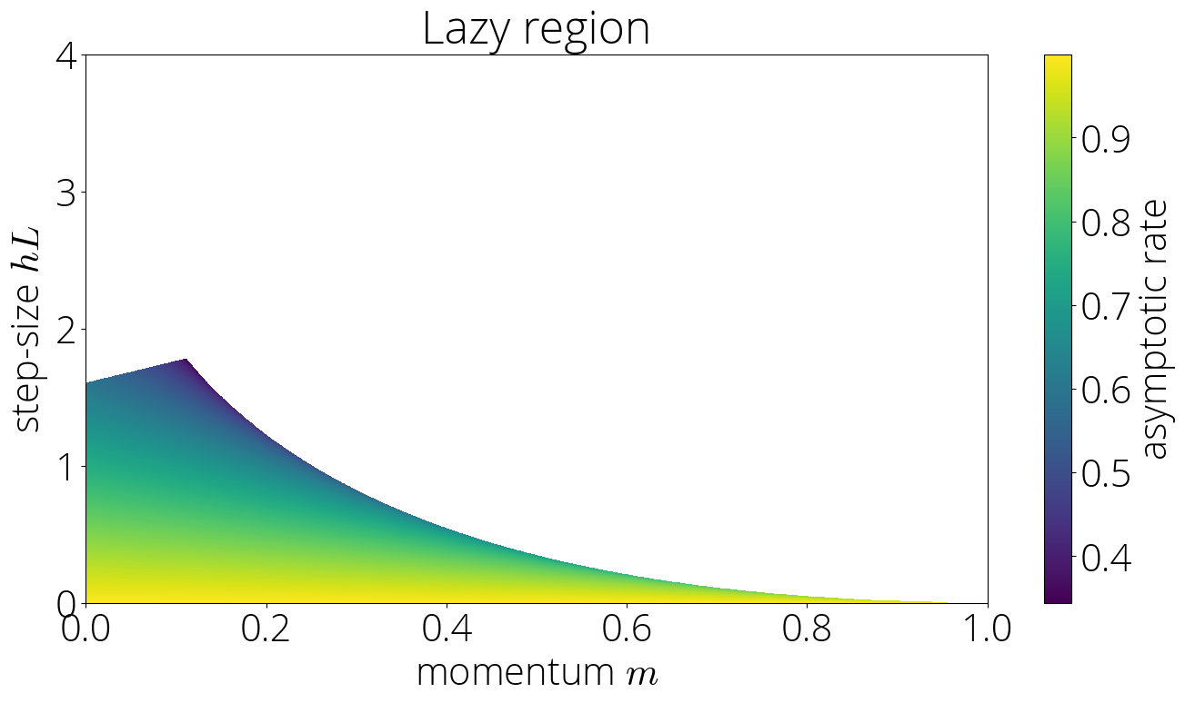
As we saw earlier, outside of the $[-1, 1]$ interval both Chebyshev have simple $t$-th root asymptotics. Using this and that both kinds of Chebyshev polynomials agree in sign outside of the $[-1, 1]$ interval we can compute the asymptotic rate as \begin{align} \lim_{t \to \infty} \sqrt[t]{r_t} &= \sqrt{\mom} \lim_{t \to \infty} \sqrt[t]{ {\small\frac{2\mom}{\mom+1}}\, T_t(\sigma(\lmin)) + {\small\frac{1 - \mom}{1 + \mom}}\,U_t(\sigma(\lmin))} \\ &= \sqrt{\mom}\left(|\sigma(\lmin)| + \sqrt{\sigma(\lmin)^2 - 1} \right) \\ \end{align} This gives the asymptotic rate for this region

In the lazy region the asymptotic rate is $r_{\infty} = \sqrt{\mom}\left(|\sigma(\lmin)| + \sqrt{\sigma(\lmin)^2 - 1} \right)$.

Unlike in the robust region, this rate depends on both the step-size and the momentum parameter, which enters in the rate through the link function $\sigma$. This can be observed in the color plot of the asymptotic rate

Knife’s Edge

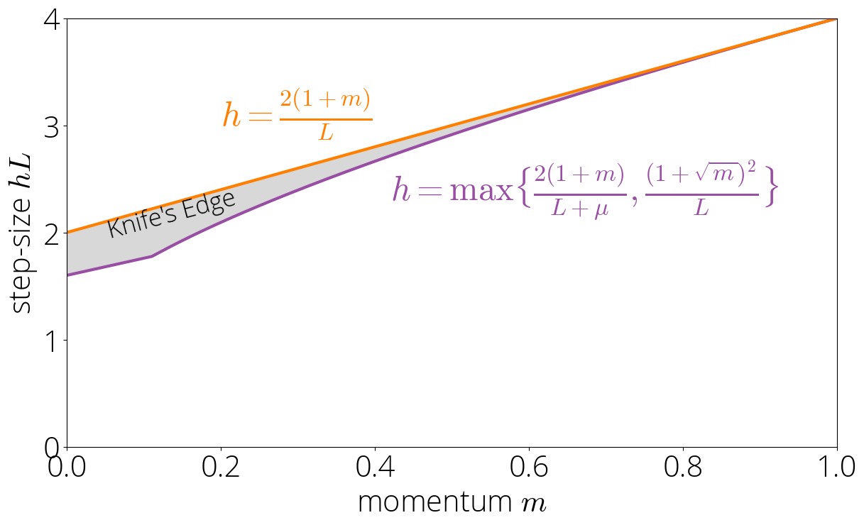
The robust and lazy region occupy most (but not all!) of the region for which momentum converges. There’s a small region that sits between the lazy and robust regions and the region where momentum diverges. We call this region the Knife’s edge

For parameters not in the robust or lazy region, we have that $|\sigma(L)| > 1$ and $|\sigma(L)| > |\sigma(\lmin)|$. Using the asymptotics of Chebyshev polynomials as we did in the previous section, we have that the asymptotic rate is $\sqrt{\mom}\left(|\sigma(L)| + \sqrt{\sigma(L)^2 - 1} \right)$. The method will only converge when this asymptotic rate is below 1. Enforcing this results in $\step \lt 2 (1 + \mom) / L$. Combining this condition with the one of not being in the robust or lazy region gives the characterization: \begin{equation} \step \lt \frac{2 (1 + \mom)}{L} \quad \text{ and } \quad \step \geq \max\Big\{\tfrac{2(1 + \mom)}{L + \lmin}, \tfrac{(1 + \sqrt{\mom})^2}{L}\Big\}\,. \end{equation}

Asymptotic rate

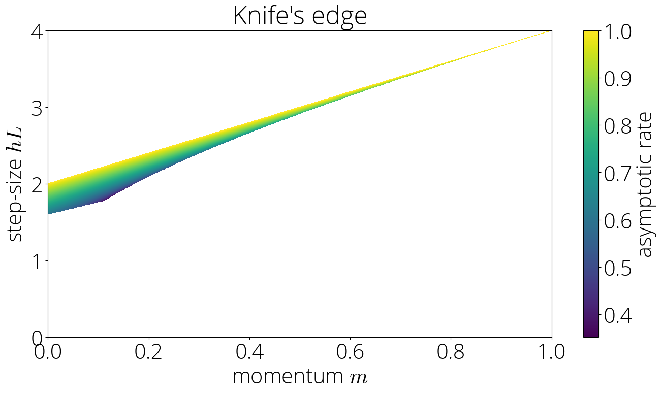
The asymptotic rate can be computed using the same technique as in the lazy region. The resulting rate is the same as in that region but with $\sigma(L)$ replacing $\sigma(\lmin)$:

In the Knife's edge region the asymptotic rate is $\sqrt{\mom}\left(|\sigma(L)| + \sqrt{\sigma(L)^2 - 1} \right)$.

Pictorially, this corresponds to

Putting it All Together

This is the end of our journey. We’ve visited all the regions on which momentum converges.There's a small convergent region with negative momentum parameter that we haven't visited. Although not typically used for minimization, negative momentum has found applications in smooth games (Gidel et al., 2020). The only thing left to do is to combine all the asymptotic rates we’ve gathered along the way.

The asymptotic rate $\limsup_{t \to \infty} \sqrt[t]{r_t}$ of momentum is \begin{alignat}{2} &\sqrt{\mom} &&\text{ if }\step \in \big[\frac{(1 - \sqrt{\mom})^2}{\lmin}, \frac{(1+\sqrt{\mom})^2}{L}\big]\\ &\sqrt{\mom}(|\sigma(\lmin)| + \sqrt{\sigma(\lmin)^2 - 1}) &&\text{ if } \step \in \big[0, \min\{\tfrac{2(1 + \mom)}{L + \lmin}, \tfrac{(1 - \sqrt{\mom})^2}{\lmin}\}\big]\\ &\sqrt{\mom}(|\sigma(L)| + \sqrt{\sigma(L)^2 - 1})&&\text{ if } \step \in \big[\max\big\{\tfrac{2(1 + \mom)}{L + \lmin}, \tfrac{(1 + \sqrt{\mom})^2}{L}\big\}, \tfrac{2 (1 + \mom) }{L} \big)\\ &\geq 1 \text{ (divergence)} && \text{ otherwise.} \end{alignat}

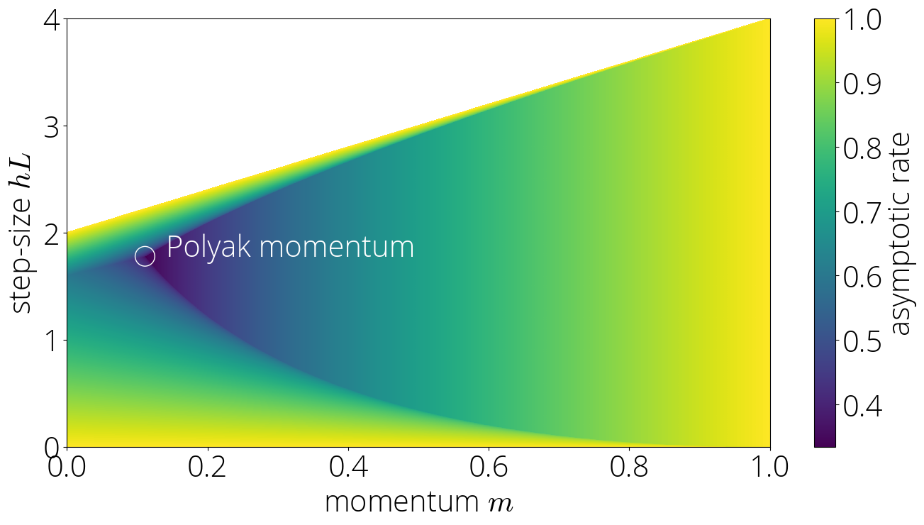
Plotting the asymptotic rates for all regions we can see that Polyak momentum (the method with momentum $\mom = \left(\frac{\sqrt{L} - \sqrt{\lmin}}{\sqrt{L} + \sqrt{\lmin}}\right)^2$ and step-size $\step = \left(\frac{2}{\sqrt{L} + \sqrt{\lmin}}\right)^2$ which is asymptotically optimal among the momentum methods with constant coefficients) is at the intersection of the three regions.

Reproducibility

All plots in this post were generated using the following Jupyer notebook: [HTML] [IPYNB]