Decay No More
Weight decay is among the most important tuning parameters to reach high accuracy for large-scale machine learning models. In this blog post, we revisit AdamW, the weight decay version of Adam, summarizing empirical findings as well as theoretical motivations from an optimization perspective.
Introduction
Weight decay is a regularization technique in machine learning which scales down the weights in every step. It dates back at least to the 1990’s and the work of Krogh and Hertz
In Pytorch, weight decay is one simple line which typically is found somewhere in the step-method:
for p in group['params']:
  p.data.add_(p.data, alpha=-decay)
Subtracting a multiple of the weight can be seen as taking a step into the negative gradient direction of the squared norm of the weight. This relates weight decay to \(\ell_2\)-regularization.
The exact mechanism of weight decay is still puzzling the machine learning community:
The story of weight decay in pictures:
— Sebastian Raschka (@rasbt) January 14, 2023
weight decay ...
1) improves data efficiency by > 50%
2) is frequently found in the best hyperparam configs
3) is among the most important hparams to tune
4) is also tricky to tune pic.twitter.com/PjWpk3pJxz
There is a gaping hole in the literature regarding the purpose of weight decay in deep learning. Nobody knows what weight decay does! AFAIK, the last comprehensive look at weight decay was this 2019 paper https://t.co/7WDBZojsm0, which argued that weight decay https://t.co/qUpCbfhFRf
— Jeremy Cohen (@deepcohen) January 22, 2023
The paper by Zhang et al. (BN)
We want to summarize two findings of
- On the one hand, weight decay has (in theory) no effect on layers with
(BN). This is simply due to the fact that(BN)makes the output invariant to a rescaling of the weights.
Weight decay is widely used in networks with Batch Normalization (Ioffe & Szegedy, 2015). In principle, weight decay regularization should have no effect in this case, since one can scale the weights by a small factor without changing the network’s predictions. Hence, it does not meaningfully constrain the network’s capacity. —Zhang et al., 2019
- However, the experiments of the paper show that weight decay on layers with
(BN)can nevertheless improve accuracy. The authors argue that this is due to an effectively larger learning rate.
This blog post will summarize the development of weight decay specifically for Adam. We try to shed some light on the following questions:
- What is the difference between Adam and its weight decay version AdamW? Does the existing literature give a clear answer to the question when (and why) AdamW performs better?
- Is the weight decay mechanism of AdamW just one more trick or can we actually motivate it from an optimization perspective?
- The last section is somewhat explorational: could we come up with different formulas for a weight decay version of Adam? By doing so, we will see that AdamW already combines several advantages for practical use.
Notation
We denote by \(\alpha > 0\) the initial learning rate. We use \(\eta_t > 0\) for a learning rate schedule multiplier. By this, the effective learning rate in iteration \(t\) is \(\alpha \eta_t\). We use \(\lambda > 0\) for the weight decay parameter.
Adam
Adam uses an exponentially moving average (EMA) of stochastic gradients, typically denoted by \(m_t\), and of the elementwise squared gradients, denoted by \(v_t\).
We denote with \(\hat m_t\) and \(\hat v_t\) the EMA estimates with bias correction (see
where \(\beta_1, \beta_2 \in [0,1)\). The update formula of Adam is given by
\[w_t = w_{t-1} - \eta_t \alpha \frac{\hat m_t}{\epsilon + \sqrt{\hat v_t}}.\]How would Adam handle regularization? The first approach to this was to simply add the regularization term \(\frac{\lambda}{2}\|w\|^2\) on top of the loss, do backpropagation and then compute the Adam step as outlined above. This is usually referred to as AdamL2. However, Loshchilov and Hutter
AdamW
For training with \(\ell_2\)-regularization, Loshchilov and Hutter proposed AdamW in 2019
While for Adam several results for convex and nonconvex problems are established fairseq library, developped by Facebook Research, which implements many SeqToSeq models. In their codebase, when Adam is specified with weight decay, AdamW is used by default (see here).
We summarize the empirical findings of
-
AdamW improves generalization as compared to AdamL2 for image classification tasks. In the paper, the authors use a ResNet model
for the CIFAR10 and Imagenet32 dataset. -
Another advantage of AdamW is stated in the abstract of
:
We provide empirical evidence that our proposed modification decouples the optimal choice of weight decay factor from the setting of the learning rate for both standard SGD and Adam [...]. —Loshchilov and Hutter, 2019
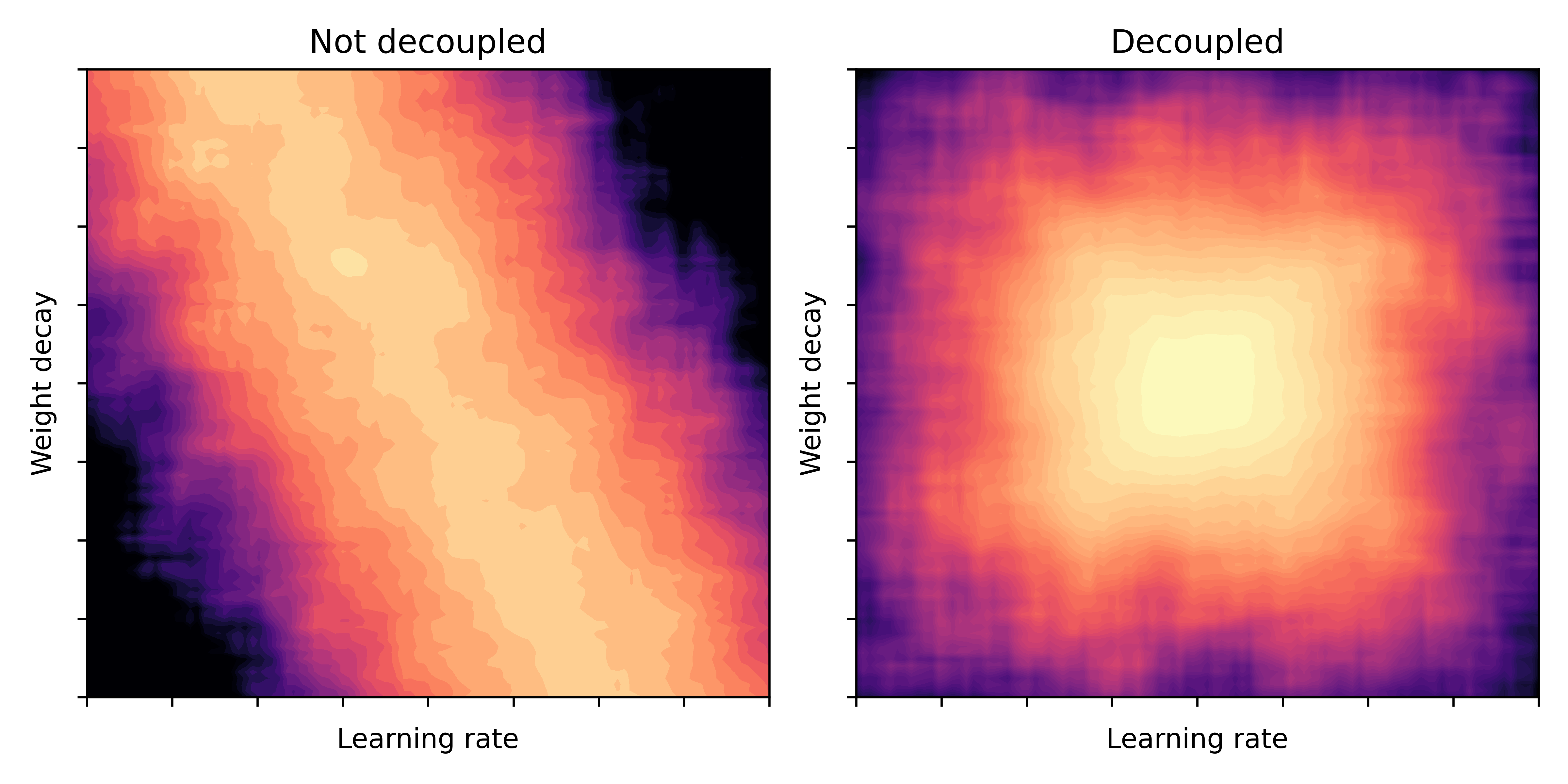
What the authors mean by decoupling is that if we plot the test accuracy as a heatmap of learning rate and weight decay, the areas with high accuracy are more rectangular; the best learing rate is not too sensitive to the choice of weight decay. We illustrate this conceptually in the plot below which is inspired by Figure 2 in

When revisiting the literature on AdamW we made an interesting practical observation: the Pytorch implementation of AdamW is actually slightly different to the algorithm proposed in the paper. In Pytorch, the following is implemented:
\[w_t = (1-\eta_t \alpha \lambda)w_{t-1} - \eta_t \alpha \frac{\hat m_t}{\epsilon + \sqrt{\hat v_t}}.\]The difference is that the decay factor in the code is \(1-\eta_t \alpha \lambda\) instead of \(1-\eta_t \lambda\) in the paper. Clearly, this is equivalent as we can simply reparametrize the weight decay factor \(\lambda\) to make up for this. However, as the default learning rate \(\alpha=0.001\) is rather small, this means that practicioners might need to choose rather high values of \(\lambda\) in order to get sufficiently strong decay. Moreover, this leaves a certain ambiguity when tuned values for \(\lambda\) are reported in the literature.
Follow-up work
In a recent article, Zhuang et al. revisit the AdamW method and try to explain its practical success
Before explaining this in detail, we first want to summarize the empirical findings of
- When
(BN)is deactivated, AdamW achieves better generalization compared to AdamL2 for image classification with a standard ResNet architecture. - When
(BN)is activated, the test accuracy of AdamW and AdamL2 are on par. Moreover, the best accuracy is achieved for no weight decay, i.e. \(\lambda=0\).
The second result is somewhat stunning as it seems to contradict the results in
Comparing the details of the experimental setups, we presume the following explanations for this:
-
The model that is trained in
is slightly different as it uses a Shake-Shake-Image ResNet . -
From Figure 4 in
, one can observe that the improvement in accuracy for the CIFAR-10 dataset becomes noticeable very late in the training (see also Section 4.3 in ). Thus, depending on the number of epochs after which training is stopped, one can reach different conclusions.
ProxAdam
The paper by Zhuang et al.
A short introduction to proximal operators
Proximal algorithms have been studied for decades in the context of (non-smooth) optimization, way before machine learning was a thing. The groundwork of this field has been laid by R. Tyrrell Rockafellar from the 1970’s onwards
If \(\varphi\) is non-smooth, we can not simply compute a gradient step - hence we have to deal with non-smooth terms in a different way. For many classical regularization functions (e.g. the \(\ell_1\)-norm), the proximal operator can be computed in closed form. This makes it a key ingredient of optimization algorithms for non-smooth, regularized problems. Assume that we want to minimize the sum of a differentiable loss \(f\) and a convex regularizer \(\varphi\), i.e.
\[\min_{w \in \mathbb{R}^n} f(w) + \varphi(w).\]The proximal gradient method in this setting has the update formula
\[w_{t} = \mathrm{prox}_{\alpha \varphi}\big(w_{t-1}- \alpha \nabla f(w_{t-1})\big),\]where \(\alpha>0\) is a step size (aka learning rate). An equivalent way of writing this (which will become useful later on) is
Weight decay as a proximal operator
For \(\ell_2\)-regularization \(\varphi(w) = \frac{\lambda}{2}\|w\|^2\), the proximal operator at \(w\) is given by \(\frac{1}{1+\lambda}w = (1-\frac{\lambda}{1+\lambda})w\). Based on this, the authors of
Knowing this, we can now understand why AdamW is approximately a proximal version of Adam. Using the first-order Taylor-approximation \(\frac{ax}{1+bx}\approx ax\) for small \(x\), applied to the coefficients in front of \(w_{t-1}\) and \(\frac{\hat m_t}{\epsilon + \sqrt{\hat v_t}}\) gives the formula
\[w_t = (1-\eta_t \lambda)w_{t-1} - \eta_t \alpha \frac{\hat m_t}{\epsilon + \sqrt{\hat v_t}}\]which is equal to AdamW. The argument we just presented is exactly how
Changing the norm
There is one more way of interpreting proximal methods. Let us begin with a simple example: Define the diagonal matrix \(D_t := \mathrm{Diag}(\epsilon + \sqrt{\hat v_t})\). Then, the Adam update can be equivalently written
In other words, Adam takes a proximal step of a linear function, but with the adaptive norm \(D_t\). This change in norm is what makes Adam different from SGD with (heavy-ball) momentum.
The update formula of ProxAdam can also be written as a proximal method:
\[\tag{P1} w_t = \mathrm{argmin}_y \langle y-w_{t-1}, \hat m_t \rangle + \frac{\lambda}{2\alpha}\|y\|_{D_t}^2 + \frac{1}{2 \eta_t \alpha}\|y-w_{t-1}\|_{D_t}^2.\]In fact, the first-order optimality conditions of (P1) are
\[0 = \hat m_t + \frac{\lambda}{\alpha} D_t w_t + \frac{1}{\eta_t \alpha}D_t (w_t-w_{t-1}).\]Solving for \(w_t\) (and doing simple algebra) gives
\[\tag{2} w_t = (1+\lambda \eta_t)^{-1}\big[w_{t-1} - \eta_t \alpha D_t^{-1} \hat m_t\big]\]which is equal to ProxAdam.
What is slightly surprising here is the term \(\alpha^{-1}\|y\|_{D_t}^2\) in (P1) - we might have expected the regularization term to be used with the standard \(\ell_2\)-norm. This leads us to our final section.
AdamW is scale-free
As an alternative to (P1), we could replace \(\alpha^{-1}\|y\|_{D_t}^2\) by \(\|y\|^2\) and update
\[w_t = \mathrm{argmin}_y \langle y-w_{t-1}, \hat m_t \rangle + \frac{\lambda}{2}\|y\|^2 + \frac{1}{2\eta_t\alpha}\|y-w_{t-1}\|_{D_t}^2.\]Again, setting the gradient of the objective to zero and solving for \(w_t\) we get
\[w_t = \big(\mathrm{Id} + \eta_t \lambda \alpha D_t^{-1}\big)^{-1} \big[w_{t-1} - \eta_t\alpha D_t^{-1} \hat m_t \big].\]Comparing this to (2) we see that the second factor is the same, but the decay factor now also depends on \(D_t\) and \(\alpha\). Let us call this method AdamP.
Now the natural question is whether AdamP or ProxAdam (or AdamW as its approximation) would be superior. One answer to this is that we would prefer a scale-free algorithm: with this we mean that if the loss function would be multiplied by a positive constant, we could still run the method with exactly the same parameters and obtain the same result. Adam for example is scale-free and in
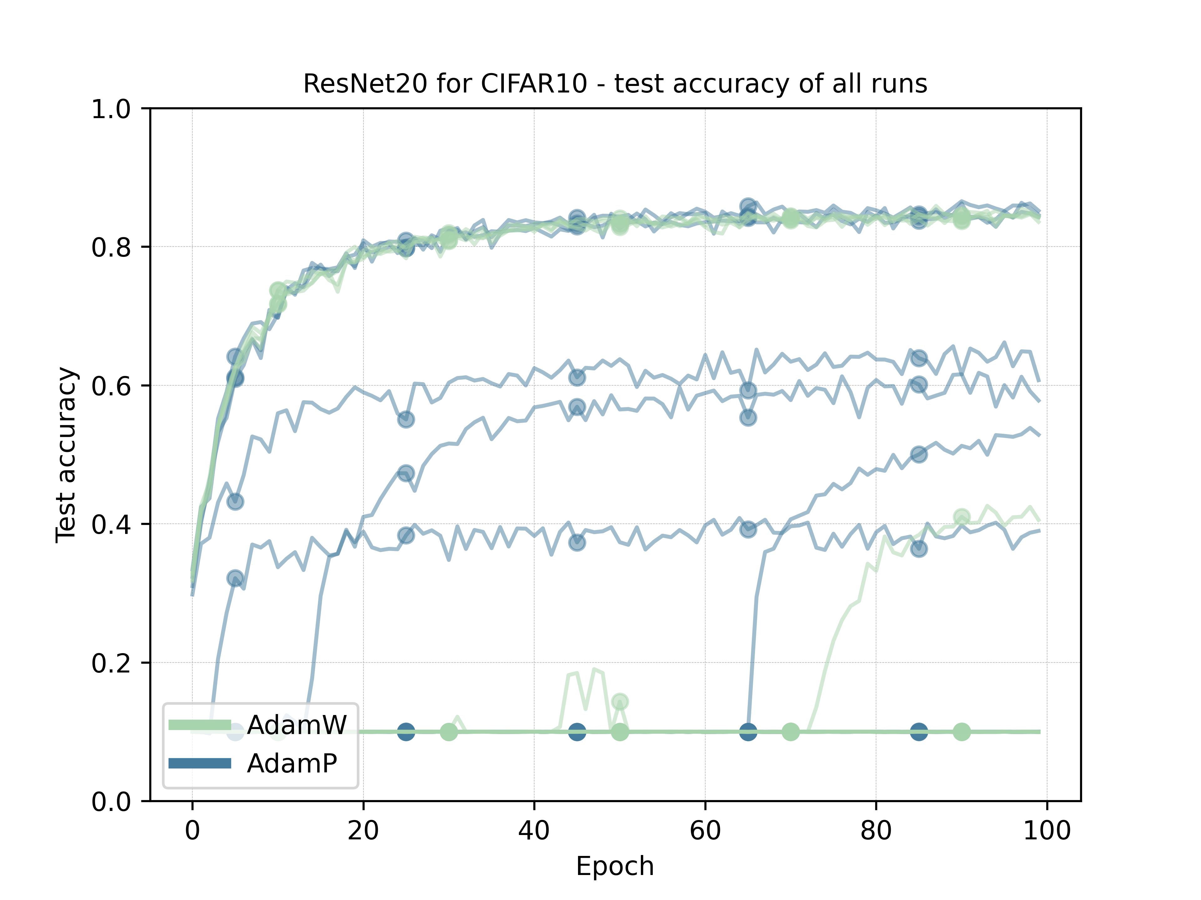
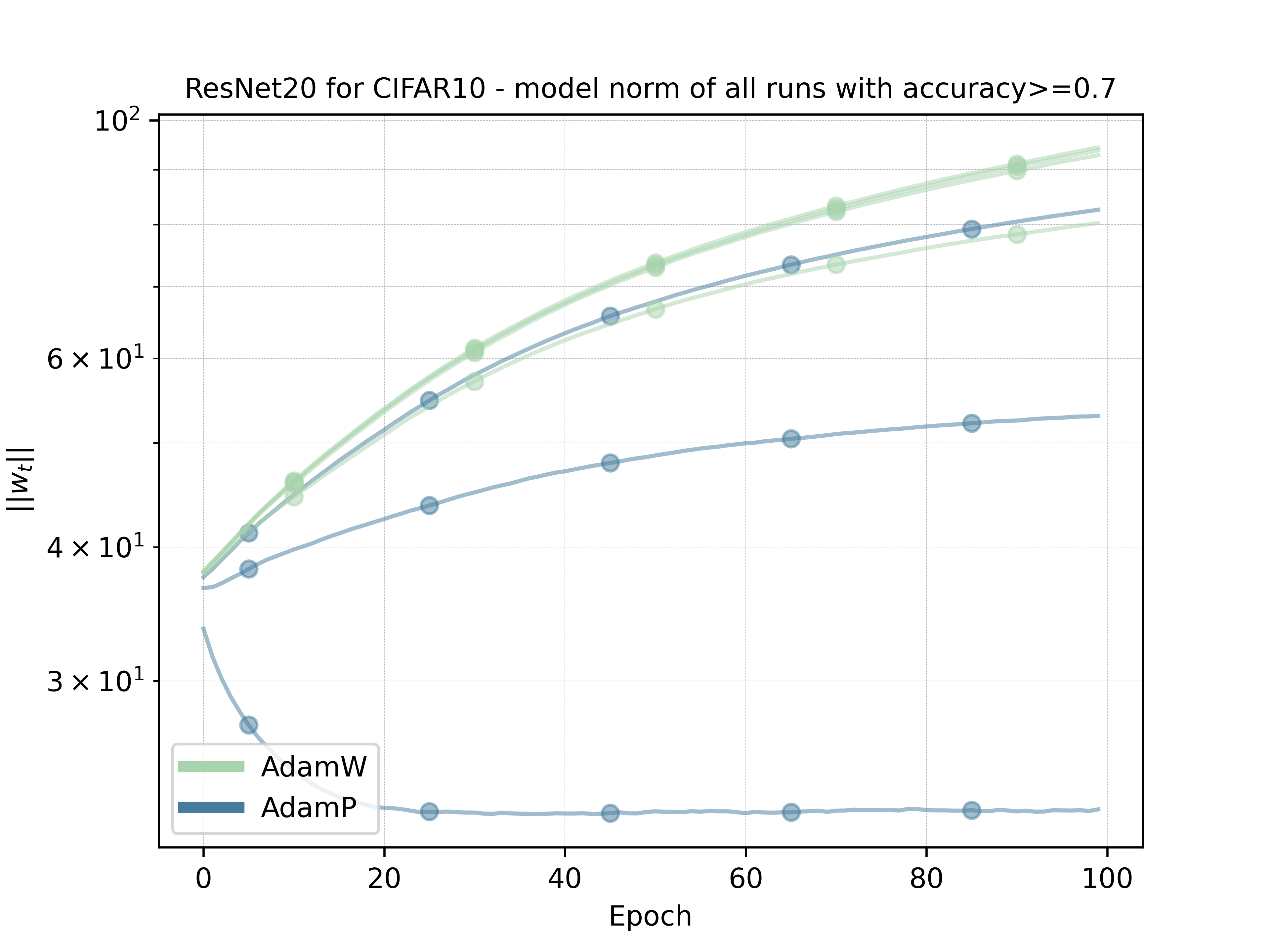
To verify this, we ran a simple experiment on a ResNet20 for CIFAR10 with (BN) deactivated. For AdamW (the Pytorch version) and AdamP we tested the learning rates [1e-3,1e-2,1e-1] and weight decay [1e-5,1e-4,1e-3,1e-2]. From the plots below, we can see that both methods approximately achieve the same accuracy for the best configurations


For the sake of completeness, we also add a Pytorch implementation of AdamP in the Appendix.
Summary
-
Weight decay can be seen as a proximal way of handling \(\ell_2\)-regularization. Therefore, it is not a different type of regularization itself but rather a different treatment of regularization in the optimization method. As a consequence, AdamW is an (almost) proximal version of Adam.
-
Whether or not weight decay brings advantages when used together with
(BN)seems to depend on several factors of the model and experimental design. However, in all experiments we discussed here AdamW performed better or at least on par to AdamL2. -
The second conclusion suggests that proximal algorithms such as AdamW seem to be favourable. Together with the scale-free property that we described in the final section, this makes AdamW a robust method and explains its practical success.
Acknowledgements
Special thanks go to Robert M. Gower and the anonymous reviewers for their constructive feedback.
Appendix
Below you find a Pytorch implementation of AdamP:
import torch
from torch.optim import Optimizer


class AdamP(Optimizer):
    r"""
    Arguments:
        params (iterable): iterable of parameters to optimize or dicts defining
            parameter groups
        lr (float, optional): learning rate (default: 1e-3)
        betas (Tuple[float, float], optional): coefficients used for computing
            running averages of gradient and its square (default: (0.9, 0.999))
        eps (float, optional): term added to the denominator to improve
            numerical stability (default: 1e-8)
        weight_decay (float, optional): weight decay (L2 penalty) (default: 0)

    """

    def __init__(self, params, lr=1e-3, betas=(0.9, 0.999), eps=1e-8,
                 weight_decay=0):
        if not 0.0 <= lr:
            raise ValueError("Invalid learning rate: {}".format(lr))
        if not 0.0 <= eps:
            raise ValueError("Invalid epsilon value: {}".format(eps))
        if not 0.0 <= betas[0] < 1.0:
            raise ValueError("Invalid beta parameter at index 0: {}".format(betas[0]))
        if not 0.0 <= betas[1] < 1.0:
            raise ValueError("Invalid beta parameter at index 1: {}".format(betas[1]))
        if not 0.0 <= weight_decay:
            raise ValueError("Invalid weight_decay value: {}".format(weight_decay))
        defaults = dict(lr=lr, betas=betas, eps=eps,
                        weight_decay=weight_decay)

        self._init_lr = lr
        super().__init__(params, defaults)

        return


    def step(self, closure=None):
        """Performs a single optimization step.

        Arguments:
            closure (callable, optional): A closure that reevaluates the model
                and returns the loss.
        """

        if closure is not None:
            with torch.enable_grad():
                loss = closure()

        for group in self.param_groups:
            for p in group['params']:
                if p.grad is None:
                    continue

                grad = p.grad
                state = self.state[p]

                # State initialization
                if 'step' not in state:
                    state['step'] = 0
                    # Exponential moving average of gradient values
                    state['exp_avg'] = torch.zeros_like(p.data).detach()
                    # Exponential moving average of squared gradient values
                    state['exp_avg_sq'] = torch.zeros_like(p.data).detach()

                exp_avg, exp_avg_sq = state['exp_avg'], state['exp_avg_sq']
                beta1, beta2 = group['betas']

                state['step'] += 1
                bias_correction1 = 1 - beta1**state['step']
                bias_correction2 = 1 - beta2**state['step']


                # Decay the first and second moment running average coefficient
                exp_avg.mul_(beta1).add_(grad, alpha= 1-beta1)
                exp_avg_sq.mul_(beta2).addcmul_(grad, grad, value= 1-beta2)
                D = (exp_avg_sq.div(bias_correction2)).sqrt().add_(group['eps'])

                lr = group['lr']
                lmbda = group['weight_decay']

                p.data.addcdiv_(exp_avg, D, value=-lr/bias_correction1)
                if lmbda > 0:
                    p.data.div_(1.0 + lr*lmbda/D) # adaptive weight decay


        return loss