How to visualize training dynamics in neural networks

Deep learning practitioners typically rely on training and validation loss curves to understand neural network training dynamics. This blog post demonstrates how classical data analysis tools like PCA and hidden Markov models can reveal how neural networks learn different data subsets and identify distinct training phases. We show that traditional statistical methods remain valuable for understanding the training dynamics of modern deep learning systems.

Introduction

What happens inside a neural network during training? Does this process unfold the same for every training run? In deep learning, the most basic way to examine training dynamics is to plot train and validation losses.

Each gradient update drives the neural network's weights towards convergence. We track this process by looking at the training loss.

Loss curves already give us some intuition about the training process. The loss starts out high because the randomly initialized weights are far from an optimal solution. Each weight update drives the network towards solving the task, and so the loss goes down.

But train and validation losses are a coarse-grained view of training dynamics. Because the validation set is sampled from the same distribution as the train set, we might miss changes in model behavior on specific data subsets or distribution shifts. Even when a change is visible, it might not be easily interpreted. For example, a bump or plateau in the training loss could have a variety of causes. If you’re training a language model, the loss increases when your model encounters a batch of gibberish data , but it also increases when your model develops a fundamental capability like in-context learning . We can’t know what caused the bump just by inspecting the loss curve.

How, then, should we interpret changes in the loss curve? One common approach is to design targeted test sets around specific tasks. Observe some interesting loss behavior, develop a hypothesis about what the model might be doing under the hood, and make or collect data that would test your hypothesis. But this is not a prescriptive approach—we basically just described the scientific method.

Instead, in this blog post, we’ll explain how to use classical data science tools to analyze training dynamics. We’ll show how to do exploratory data analysis on training dynamics first. Test tasks can come later—right now, we want a more fine-grained, bottom-up description of how our neural networks learn.

A Motivating Example: Grokking Modular Addition

Let’s start with a simple example: teaching a neural network to perform modular addition. Specifically, we’ll train a small language model to compute (x + y) mod 113 = z. (We use mod to ensure the sum lands within the existing language model’s token embedings.) Modular addition, studied in the grokking literature, exhibits interesting training dynamics that make it perfect for our analysis.

Input: (x, y) where x, y ∈ [0, 112]
Output: z, where z = (x + y) mod 113
Model: Single-layer Transformer
Dataset: 80% train, 20% validation

Modular addition task details. Training on modular addition leads to the grokking phenomenon, where the language model suddenly learns to generalize after many epochs of high validation loss.

In particular, if we plot the training and validation losses, we see something curious:

• Initially, both losses are high as the model starts from random weights.
• Memorization: Training loss then drops to near-zero quickly, but validation loss remains high or increases.
• Generalization: After a long period of gradual decline, the validation loss suddenly drops—the model has “grokked” the task.

This runs counter to the traditional train-validation loss behavior in machine learning, where the training and validation loss tend to drop in tandem, and validation loss eventually begins rising when the model overfits.

We now understand this phenomenon quite well. One explanation is that there exist competing subnetworks in the model—one that tries to memorize the training data, and another that implements the correct mathematical function. Initially, the memorization subnetwork dominates, but with enough training, the generalizing subnetwork eventually takes over, leading to sudden improvement in the validation loss .

Here, we will use modular addition both to validate our data analysis methods and for pedagogical purposes. The dramatic phase transition from memorization to generalization makes it easy to see whether our methods are working—if they can’t detect this clear shift, they likely won’t catch subtler changes. At the same time, this clear transition makes it easy to understand how each analysis technique reveals different aspects of training dynamics.

PCA: Analyzing Sequences of Functions

Beyond examining aggregate training or validation losses, we can visualize how the neural network’s implemented function—its mapping from inputs to outputs—evolves over time. Principal Component Analysis (PCA) offers one way to do this. Suppose we’ve saved some checkpoints of weights \(\theta_{1:T}\) throughout training. Then, we can:

• Choose a (random) subset of sample inputs (x₁, y₁), (x₂, y₂), …, (xₙ, yₙ).
• At each checkpoint \(\theta_i\), compute the loss for each sample. This yields an \(n\)-dimensional loss vector, where \(n\) is the number of samples.
• Apply PCA to these vectors to get a lower-dimensional representation, and visualize.

Why use PCA? Consider a scenario where your model learns half of the dataset first, then the other half. In this case, PCA would likely reveal two large principal components, since your loss vector can be represented with a 2D vector—one dimension for the first half, and one dimension for the second. Thus, tracking your model’s trajectory in PCA space reveals how it learns different data subsets, even without knowing exactly what these subsets are.

We treat the losses on a subset of training samples as a representation of the function. We can reduce the dimensionality of this representation using PCA and visualize.

Let’s test this approach on our modular addition example. We trained a one-layer transformer for 500 epochs on the modular addition task. At each checkpoint, we computed losses on a fixed subset of the validation set to obtain our \(n\)-dimensional vector. Then we applied PCA to the entire sequence of vectors.

If you mouse over the points in the figure, you’ll find that the direction change in the PCA plot exactly corresponds to when the validation loss drops sharply to zero, or when the model starts to generalize! Before grokking occurs, the model gets high losses on validation samples that can’t be solved through memorization. When grokking occurs, the losses on these examples start to drop, resulting in the direction change in the PCA plot.

For a deeper dive on this approach and analyses stemming from PCA, see “The Developmental Landscape of In-Context Learning” by Hoogland et al. (2024).

Summary: Use PCA to explore loss behaviors. Principal components can relate to changes in model behavior on data subsets.

HMM: Analyzing Sequences of Weights

We can also analyze the neural network’s weights to understand training dynamics. While the previous section focused on PCA, here we’ll explore using clustering to group neural network checkpoints into distinct phases, rather than treating them as a continuous sequence. By identifying distinct phases of learning, we can analyse each phase independently—for instance, by investigating what capabilities a model develops in each phase. The simplest method that comes to mind is K-means clustering, but K-means cannot account for temporal relationships, or the fact that our checkpoints occur in a sequence.

Instead, we can use a hidden Markov model (HMM), which does model temporal dependencies. While we could apply the HMM to the sequence of loss vectors from the previous section, we’re also interested in how the weights themselves evolve. We can’t simply run PCA on the weights—they’re typically too high-dimensional.

The paper “Latent State Models of Training Dynamics” offers a solution: compute various metrics over the weights, such as the average \(L_2\) norm and largest eigenvalue of the weight matrices. As Hu et al. (2023) demonstrate, we can hand-craft a dimensionality reduction by selecting metrics that capture different aspects of the weights.

Concretely, here’s the procedure. For a neural network with weight matrices \(\{ w_i \}_{1:N}\):

• At each checkpoint, collect metrics about the weights, such as:
  • Average L2 norm of weights: \(\frac{1}{N} \sum_{i=1}^{N}|| w_i ||_2\)
  • Average largest eigenvalue: \(\frac{1}{N} \sum_{i=1}^{N} \lambda_{\texttt{max}}( w_i )\)
• Fit a hidden Markov model (HMM) to these sequences of metrics.

Here, we perform dimensionality reduction by collecting several metrics about the weights, such as their norms, means, and variances. We then train a hidden Markov model (HMM) to predict the sequence of statistics.

After fitting the HMM, we can cluster checkpoints by predicting each checkpoint’s hidden state. Below, we’ve taken our modular addition training trajectory from the previous section, computed weight metrics for each checkpoint, and trained an HMM to predict these metrics. The HMM’s hidden states are shown in different colors, with a graphical representation of the model on the right.

The HMM identifies distinct phases in training by analyzing sequences of weight statistics. These phases can be used to cluster checkpoints and analyze new training trajectories.

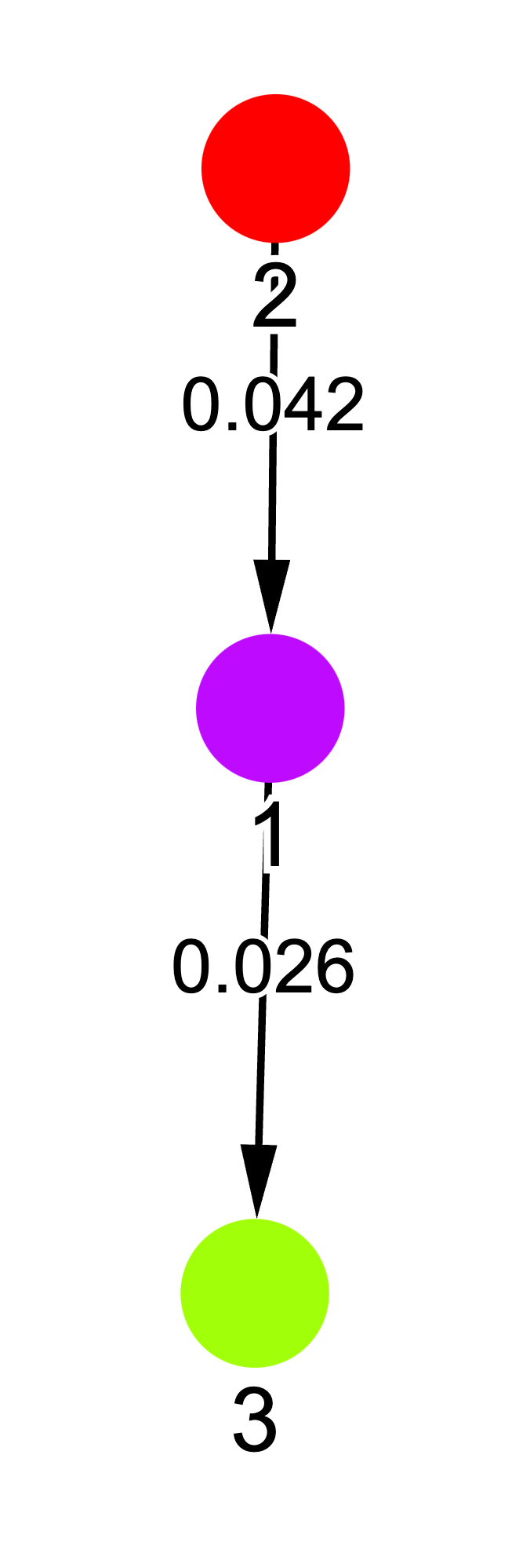
We notice that the HMM segments training into three phases, which roughly align with the memorization, generalization, and convergence phases in grokking. This is interesting because the HMM only sees weight statistics—it has no access to loss values. Thus, the behavioral changes we observe in the loss curves are reflected in the underlying weight dynamics. For a deeper dive on using HMMs to analyze training dynamics, see Hu et al. (2023).

Summary: Use the hidden Markov model to cluster checkpoints. Clusters can reflect changes in the model or phase transitions.

Conclusion

Classical data analysis tools like PCA and HMMs can provide insights into neural network training dynamics. In this blog post, we demonstrated two complementary approaches: using PCA to visualize how models learn different subsets of data over time, even without explicitly identifying these subsets, and applying HMMs to discover distinct phases in training by analyzing weight statistics. Applied to the grokking phenomenon, these methods revealed clear phase transitions—from memorization to generalization to convergence—with the HMM discovering these phases purely from weight dynamics, without access to loss values.

These results suggest that traditional statistical methods remain valuable tools for understanding modern deep learning systems. While neural networks may seem dauntingly complex, careful application of classical analysis techniques can help us better understand their training process. Code to reproduce this blog post is here.