SPD Attack - Prevention of AI Powered Image Editing by Image Immunization
Recent advances in image-to-image editing models offer both benefits and risks. While they enhance creativity, accessibility, and applications in fields ranging from medicine to environmental science, they can also enable misuse, such as identity manipulation, copyright infringement, and deepfake creation. This blog explores methods to protect images from such misuse, reproduces findings from relevant research, and extends them across various models and datasets.
AI image editing tools are becoming incredibly powerful and easy to use. With just a few clicks, these tools can transform images in ways that used to take hours of expert work. While this technology opens up amazing creative possibilities and makes advanced editing accessible to everyone, it also creates new risks. Images can be manipulated to create misleading content, fake identities, or violate artists’ rights.
This blog introduces Safeguarded Perturbation Defense (SPD) Attack, a new way to “immunize” images against AI manipulation. Our method builds on recent works that immunize images against adversarial attackers. Particularly, Immunization is achieved by adding subtle, imperceptible perturbations into images, reinforcing their resistance to unintended image editing. These perturbations interfere with the functionality of generative models, inhibiting image manipulation while preserving the original visual characteristics and perceptual fidelity.
Current methods generate a single adversarial noise to a single image, in our blog we explore how to extend these approaches for multiple images.
Background
Diffusion Models
Diffusion Models are a class of probabilistic generative models that learn to approximate a data distribution $p(x)$ by gradually denoising a normally-distributed variable. These models define a Markov chain of diffusion steps to slowly add random noise to a sample from the data distribution $q(x)$ and then learn to reverse the diffusion process to construct desired samples from the target distribution $p(x)$ from the noisy sample.
Forward Diffusion Process
Given a data point $x_0 \sim q(x_0 )$, the forward diffusion process adds small noise typically gaussian to the given data point for T steps according to the distribution $q(x_t | x_{t-1})$ to produce the noisy samples $x_1 , x_2 ,…..x_T$. The step sizes $\beta_t$ control the amount of noise at each step and they are controlled by a variance scheduler.
\[q(x_t | x_{t-1}) = \mathcal{N}(x_t;\sqrt{1-\beta_t}x_{t-1},\beta_t \mathbf{I})\]Reverse Diffusion Process
Given the final output $x_T$, the reverse diffusion process learns to sample from $q(x_{t-1} | x_t,x_0)$ to create the desired sample. We learn to model $p_{\theta}(x_{t-1} | x_t)$ to approximate this conditional distribution using a normal distribution.
\[p_{\theta}(x_{t-1} | x_t)=\mathcal{N}(x_{t-1};\boldsymbol{\mu}_{\theta}(x_t,t),\boldsymbol{\Sigma}_{\theta}(x_t,t))\]Ho et al. 2020
Latent Diffusion Models
In this blog, we will specifically focus on Latent Diffusion Models Rombach et al. 2022
LDM uses an encoder network $\mathcal{E}$ to map the original input image $x_0$ to its latent representation $z_0 = \mathcal{E}(x_0)$, the diffusion process is then trained on this latent space to obtain $\tilde{z}$, and the final output $\tilde{x}$ is obtained by decoding $\tilde{z}$ using the corresponding decoder network $\mathcal{D}$.
Variational Autoencoder
VAEs
Adversarial attacks
In computer vision tasks, an adversarial example is an imperceptible perturbation of that image formed by applying small but intentionally worst-case perturbations to examples from the dataset, such that the perturbed input results in the model outputting an incorrect answer with high confidence
Here, $\Delta$ represents the set of perturbations that are small enough that they are imperceptible, i.e. $\Delta = { \delta : | \delta |_p \leq \epsilon }$ according to some $L_p$ norm. The most common approach to solve this optimization problem is using projected gradient descent (PGD)
Universal Adversarial Perturbations (UAPs)
Universal Adversarial Perturbations (UAPs)
The perturbation \(\delta\_{u}\) is designed to satisfy the following criteria:
-
Universality: The perturbation should work for most input samples \(x \sim q(x)\), i.e.,
\[P_{x \sim q(x)}[f_\theta(x + \delta_u) \neq f_\theta(x)] \geq \tau\]where \(\tau\) is a desired success rate threshold.
-
Imperceptibility: The perturbation must remain small enough to be imperceptible to a human observer, typically constrained by an \(L_p\)-norm such that \(\|\delta_u\|\_p \leq \epsilon\).
-
Generalization: The perturbation should generalize across different inputs rather than being tailored to a specific sample.
Finding UAPs
The UAP optimization problem can be expressed as:
\[\delta_u = \arg \min_{\delta \in \Delta} \mathbb{E}_{x \sim q(x)}[L(f_\theta(x + \delta), f_\theta(x))]\]Here:
- \(\Delta = \{\delta : \|\delta\|\_p \leq \epsilon \}\) represents the constraint on imperceptibility.
- \(L(\cdot)\) is the loss function capturing misclassification.
Related Work
Photoguard
Photoguard
Encoder Attack
This attack primarily focuses on manipulating the latent representation of an image encoded by a VAE encoder. By adding specific noise to the original image, it maps the image to a “bad” latent representation, which ultimately disrupts downstream tasks and results in an overall distorted image.
The researchers used a simple optimization approach to bring the latent space embedding closer to the target latent space using PGD. If $\delta_{encoder}$ represents the noise added to the original image, it can be formulated as:
\[\delta_{\text{encoder}} = \arg \min_{\|\delta\|_{\infty} \leq \epsilon} \left\| \mathcal{E}(\mathbf{x} + \delta) - \mathbf{z}_{\text{targ}} \right\|_2^2\]Diffusion Attack
This attack targets the complete LDM pipeline (VAE + Denoising Model) to optimize the noise so that the generated image is closer to the target image.
The perturbation in the original image $\delta_{diffusion}$ can be calculated by:
\[\delta_{\text{diffusion}} = \arg \min_{\|\delta\|_{\infty} \leq \epsilon} \left\| f(\mathbf{x} + \delta) - \mathbf{x}_{\text{targ}} \right\|_2^2\]This approach is much powerful than the encoder attack, since it targets the text conditioning part as well but it demands significant computational resources, as we backpropagate through multiple models to calculate the gradient.
AdvDM and SDS
Motivation
For a diffusion model $\theta$, AdvDM’s
Attack
Given a diffusion model parameterized by $\theta$ and the distribution of real data $q(x)$, the adversarial example $x^{‘}$ is formulated by $x^{‘}=x+\delta$, where $x \sim q(x)$ and $\delta$ is given by the following equation:
\[\delta := \arg \min_\delta \mathbb{E}_{x^{'}_{1:T} \sim u(x^{'}_{1:T})} p_\theta(x^{'}_{0:T}) = \arg \max_\delta \mathbb{E}_{x^{'}_{1:T} \sim u(x^{'}_{1:T})} \mathcal{L}_{DM}(x^{'}, \theta)\]Where \(x^{'}_{1:T}\) the forward diffusion’s sampling steps and \(x^{'}_{1:T} \sim u(x^{'}_{1:T})\) and \(\mathcal{L}_{DM}(x^{'}, \theta)\) represents the noise estimation loss (also known as semantic loss) used during the training of LDM as shown below.
\[\mathcal{L}_{DM}(x,\theta)=\mathbb{E}_{t, \epsilon} \mathbb{E}_{z_t \sim q_t\left(\mathcal{E}_\phi(x)\right)} \| \epsilon_{\theta}(z_t,t)-\epsilon \|_2^2\]Building upon AdvDM, Xue et al. 2024
SDS Attack
Using the same attack setting as AdvDM, SDS modifies the optimization problem as follows:
\[\delta :=\arg \min_\delta \mathbb{E}_{x^{'}_{1:T} \sim u(x^{'}_{1:T})} \mathcal{L}_{DM}(x^{'}, \theta)\]Score Distillation Sampling
In practice, gradients from U-Net are expensive to compute, and poorly conditioned for small noise levels as it is trained to approximate the scaled Hessian of the marginal density. Poole et al. 2022
SDS uses this idea for faster and cheaper gradient computation to solve the optimization problem mentioned above.
Notably, The authors introduce 4 new attacks:
- AdvDM(-): Minimizing $L_{DM}$ using classical gradient computation.
- SDS(+): Maximizing $L_{DM}$ using Score Distilling Sampling.
- SDS(-): Minimizing $L_{DM}$ using Score Distilling Sampling.
- SDST: Minimizing $L_{T}$ (Photoguard) using Score Distilling Sampling.
PCA
Due to the dominance of the KL Divergence term in the learning objective, training of VAE usually suffers an optimization issue called posterior collapse
Attack
Instead of optimizing the latent space towards a grey noise as done by Photoguard
This paper proposed two methods two attack the image both of which essentially use the following loss function in different regards
\[\mathcal{L}_{\text{KL}}(x) = D_{\text{KL}}\left( q(z|x) \parallel p^*(z) \right) = \frac{1}{2} \sum_{i=1}^{d} \left( \frac{\sigma_i^2 + \mu_i^2}{v} - 1 + \ln \frac{v}{\sigma_i^2} \right).\]Where $p^*(z) \sim \mathcal{N}(0, v)$ where $v$ controls the disruptive effect of the attack
PCA+ Attack
In this attack the latent distribution is pushed away from prior distribution $\mathcal{N}(0, v)$ to create out-of-distribution scenarios eventually destroying the latent representation and further downstream tasks. The attack can be given by :
\[\max_{\delta} \mathcal{L}_{\text{KL}}(x + \delta) \quad \text{s.t.} \quad \|\delta\|_{\infty} < \epsilon.\]For $v = 1$ the loss function becomes
\[\mathcal{L}_{\text{KL}}(x) = \frac{1}{2} \sum_{i=1}^d \left( -\ln \sigma_i^2 - 1 + \mu_i^2 + \sigma_i^2 \right)\]where $\delta$ is the noise added to image $x$, the resulting image $x + \delta$ can be crafted using PGD attack. Maximizing the given loss leads to $\sigma_i^2 \rightarrow \infty$ and $\mu_i^2 \rightarrow \infty$
PCA- Attack
Instead of taking it out-of-distribution this attack is closer to Photoguard, wherein the latent distribution is forced closer to a “zero” distribution i.e. $p^*(z) \sim \mathcal{N}(0, 0)$. This optimization can be formulated by :
\[\min_{\delta} \mathcal{L}_{\text{KL}}(x + \delta) \quad \text{s.t.} \quad \|\delta\|_{\infty} < \epsilon, v \approx 0\]In this case $\mathcal{L}_{\text{KL}}(x + \delta)$ can be approximated as
\[\mathcal{L}_{\text{KL}}(x + \delta) = \sum_{i=1}^{d} \frac{\sigma_i^2 + \mu_i^2}{v}\]So if $v \rightarrow 0^+$ minimizing the term will result in $\sigma_i^2 \rightarrow 0$ and $\mu_i^2 \rightarrow 0$ eventually collapsing the distribution to a Dirac Distribution thus distorting the latent representation.
SPD-Attack: Universal Adversarial Perturbations for Photoguard and PCA
In this section we discuss our attack called *SPD-Attack. The SPD-Attack generalizes Universal Adversarial Perturbations (UAP’s) to disrupt the functionalities of diffusion-based pipelines (e.g., *Photoguard) and address latent-space vulnerabilities like those leveraged in Posterior Collapse Attacks (PCA). By applying the concept of Universal Adversarial Perturbations (UAPs), SPD-Attack finds a single perturbation that generalizes across inputs, enabling efficient and widespread disruption.
Formulation
Given a dataset \(X = \{x*1, x_2, \dots, x_n\}\), the objective is to compute a universal perturbation \(\delta*{\text{u}}\) that disrupts the encoder, diffusion, or latent representation mechanisms across most inputs \(x_i \in X\).
Encoder Attack (Photoguard)
The universal perturbation for the Encoder Attack targets the latent representation \(z\_{\text{targ}}\) and is computed as:
\[\delta_{\text{u}} = \arg \min_{\|\delta\|_p \leq \epsilon} \mathbb{E}_{x \sim q(x)} \left[ \left\| \mathcal{E}(x + \delta) - z_{\text{targ}} \right\|_2^2 \right],\]where \(\mathcal{E}\) is the encoder, and \(z\_{\text{targ}}\) disrupts downstream tasks or leads to undesirable outputs.
PCA Attack
For Posterior Collapse Attack (PCA), the universal perturbation exploits the KL divergence term in the VAE loss to disrupt the latent space and induce posterior collapse.
-
PCA+ Attack: Pushes the latent representation away from the prior distribution, creating out-of-distribution scenarios. The universal perturbation \(\delta\_{\text{u}}\) is formulated as:
\[\delta_{\text{u}} = \arg \max_{\|\delta\|_p \leq \epsilon} \mathbb{E}_{x \sim q(x)} \mathcal{L}_{\text{KL}}(x + \delta),\]where \(\mathcal{L}\_{\text{KL}}(x + \delta)\) is the KL divergence:
\[\mathcal{L}_{\text{KL}}(x) = \frac{1}{2} \sum_{i=1}^d \left( -\ln \sigma_i^2 - 1 + \mu_i^2 + \sigma_i^2 \right).\]This forces \(\sigma_i^2 \to \infty\) and \(\mu_i^2 \to \infty\), leading to highly distorted latent distributions.
-
PCA- Attack: Collapses the latent representation towards a degenerate prior \(\mathcal{N}(0, 0)\). The universal perturbation is formulated as:
\[\delta_{\text{u}} = \arg \min_{\|\delta\|_p \leq \epsilon} \mathbb{E}_{x \sim q(x)} \mathcal{L}_{\text{KL}}(x + \delta),\]where minimizing \(\mathcal{L}\_{\text{KL}}(x)\) results in \(\sigma_i^2 \to 0\) and \(\mu_i^2 \to 0\), effectively collapsing the posterior distribution.
Optimization Strategies for Multiple Images
To craft the universal perturbation \(\delta\_{\text{u}}\), we employ iterative optimization methods that ensure imperceptibility while effectively disrupting the targeted system. The two strategies that we used are Projected Gradient Descent (PGD)
1. Projected Gradient Descent (PGD)
Algorithm:
- Initialization: Initialize the perturbation \(\delta*{\text{u}} = 0\) or random noise satisfying \(\|\delta*{\text{u}}\|\_p \leq \epsilon\).
- Iterative Updates:
- For each iteration \(t\):
- Compute the loss \(L(x*i, \delta*{\text{u}})\) for each sample \(x_i\) in the dataset.
- Compute the gradient for each sample: \(g_i = \nabla_\delta L(x_i, \delta_{\text{u}}).\)
- Aggregate the gradients by taking the mean: \(\bar{g} = \frac{1}{n} \sum_{i=1}^n g_i.\)
- Update the perturbation: \(\delta_{\text{u}} \leftarrow \delta_{\text{u}} - \eta \cdot \text{sign}(\bar{g}).\)
- Project \(\delta\_{\text{u}}\) back into the \(\ell_p\)-norm constraint: \(\delta_{\text{u}} \leftarrow \Pi_{\|\delta\|_p \leq \epsilon}(\delta_{\text{u}}).\)
- For each iteration \(t\):
- Convergence: Repeat until the loss converges or the maximum number of iterations is reached.
2. Adam Optimizer
Algorithm:
- Initialization: Initialize \(\delta*{\text{u}} = 0\) or random noise satisfying \(\|\delta*{\text{u}}\|\_p \leq \epsilon\). Initialize first and second moment estimates \(m_0\) and \(v_0\).
- Iterative Updates:
- For each iteration \(t\):
- Compute the loss \(L(x*i, \delta*{\text{u}})\) for each sample \(x_i\) in the dataset.
- Compute the gradient for each sample: \(g_i = \nabla_\delta L(x_i, \delta_{\text{u}}).\)
- Aggregate the gradients by taking the mean: \(\bar{g} = \frac{1}{n} \sum_{i=1}^n g_i.\)
- Update the first and second moment estimates: \(m_t = \beta_1 m_{t-1} + (1 - \beta_1) \bar{g}, \quad v_t = \beta_2 v_{t-1} + (1 - \beta_2) \bar{g}^2.\)
- Compute bias-corrected estimates: \(\hat{m}_t = \frac{m_t}{1 - \beta_1^t}, \quad \hat{v}_t = \frac{v_t}{1 - \beta_2^t}.\)
- Update the perturbation: \(\delta_{\text{u}} \leftarrow \delta_{\text{u}} - \eta \cdot \frac{\hat{m}t}{\sqrt{\hat{v}_t} + \epsilon_{\text{adam}}}.\)
- Project \(\delta\_{\text{u}}\) back into the \(\ell_p\)-norm constraint: \(\delta_{\text{u}} \leftarrow \Pi_{\|\delta\|_p \leq \epsilon}(\delta_{\text{u}}).\)
- For each iteration \(t\):
- Convergence: Repeat until the loss converges or the maximum number of iterations is reached.
For both the optimization stratagies, the loss function can be same.
Experimental Setup
We adopted an experimental setup similar to PCA, utilizing the Stable Diffusion 1.5 Latent Diffusion Model (LDM) pipeline for all experiments.
Dataset and Model
A subset of 100 images from the ImageNet dataset was used. The images were split into training and testing sets with a ratio of 64:36 and resized to a uniform resolution of $512 \times 512$.
Baseline and Attack
The baseline was constructed using random uniform noise with $\epsilon = (4, 13, 22, 31, 40)/255$ applied to both training and testing images. For the attack, the same $\epsilon$ values were used, with 500 iterations conducted for each $\epsilon$. The following prompts were used:
• P1: “make it like a watercolor painting”
• P2: “apply sunset lighting”
• P3: “add some snow”
• P4: (empty prompt)
Image Quality Assessment
We evaluated image quality using the following metrics:
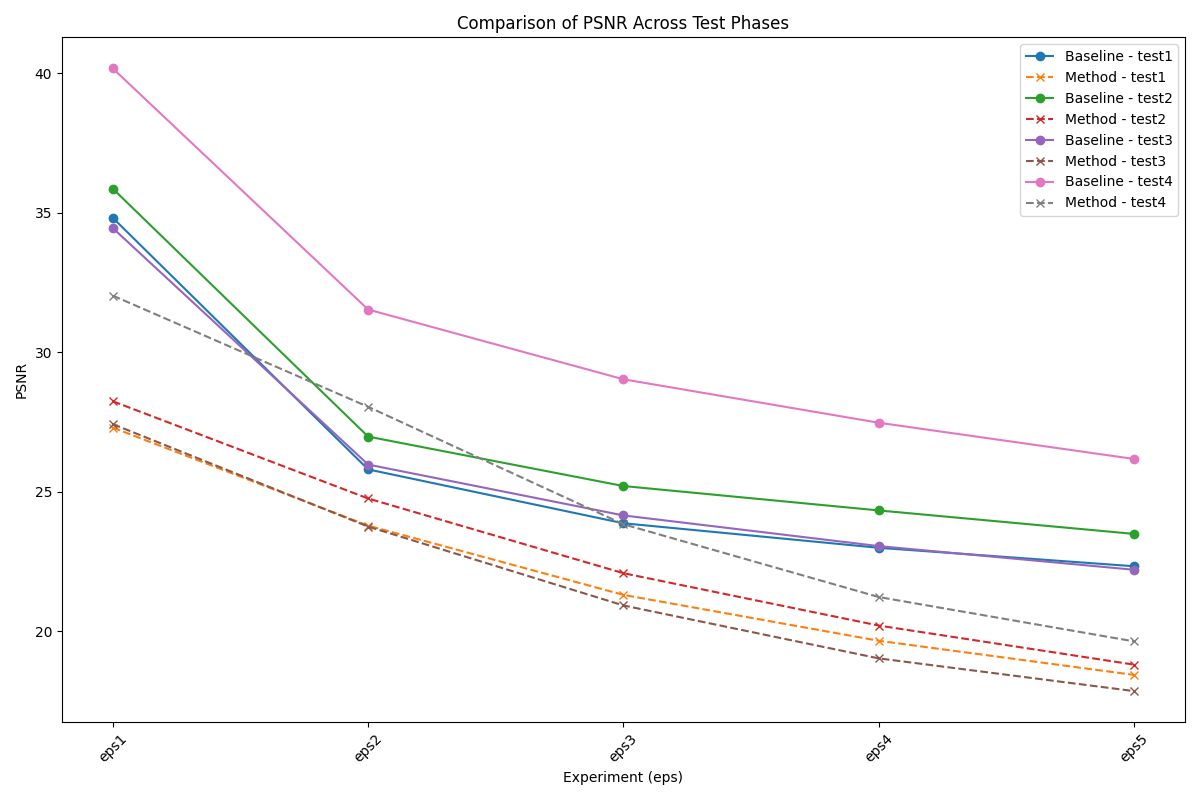
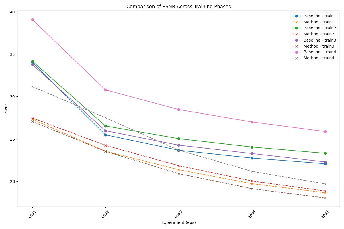
• Peak Signal-to-Noise Ratio (PSNR) : Provides insights into the overall distortion introduced in the image.
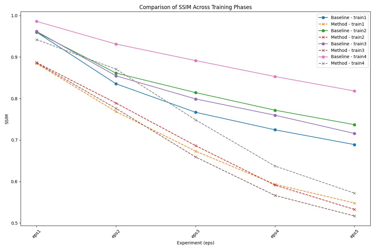
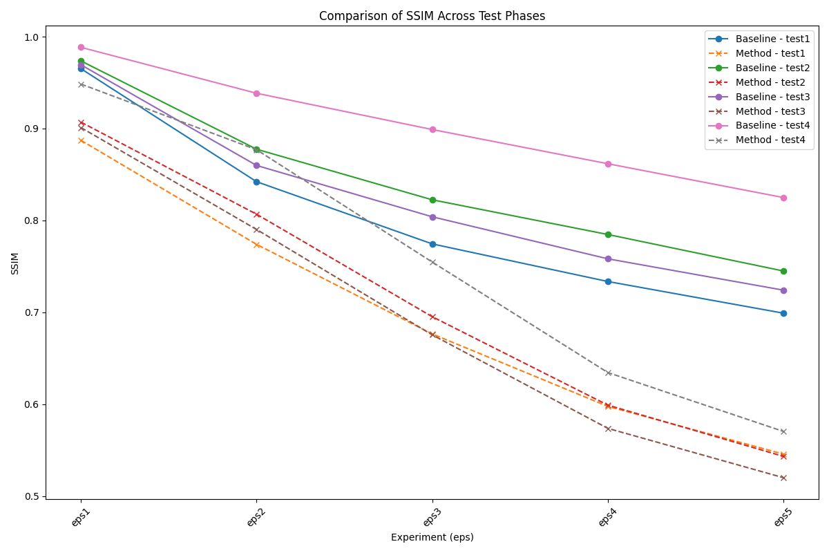
• Structural Similarity Index (SSIM) : Measures changes in local patterns of pixel intensities, emphasizing perceptual quality.
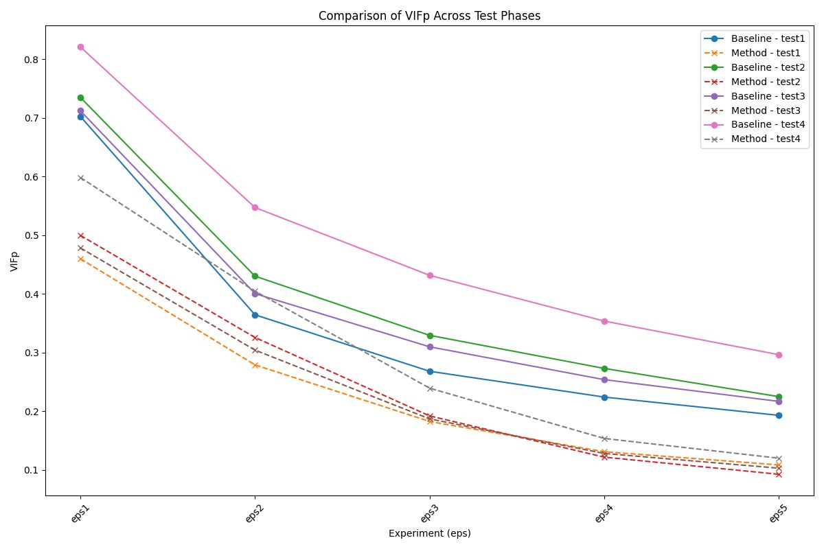
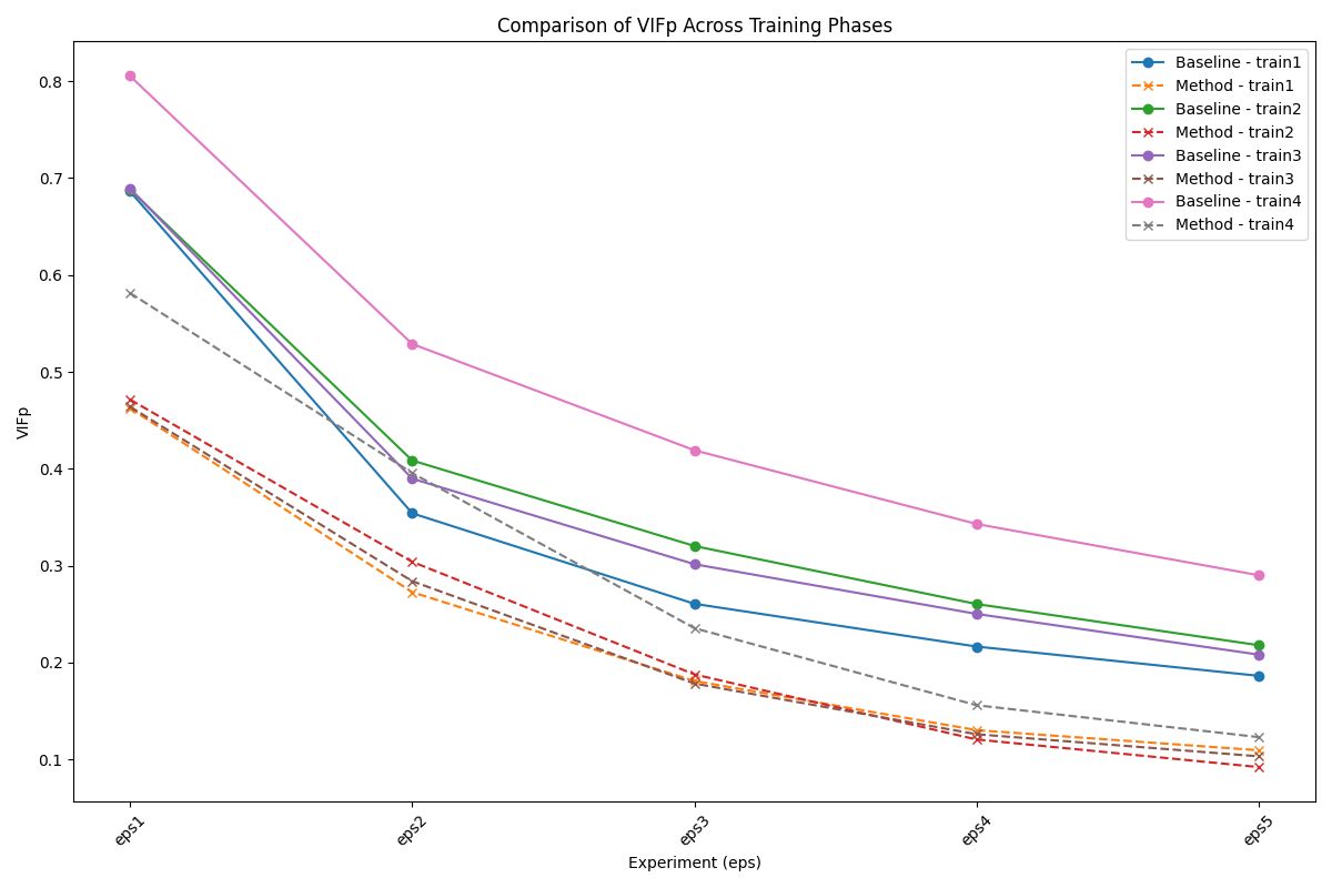
• Visual Information Fidelity in the Pixel Domain (VIFP) : Assesses image quality based on the similarity of statistical information between reference and distorted images.
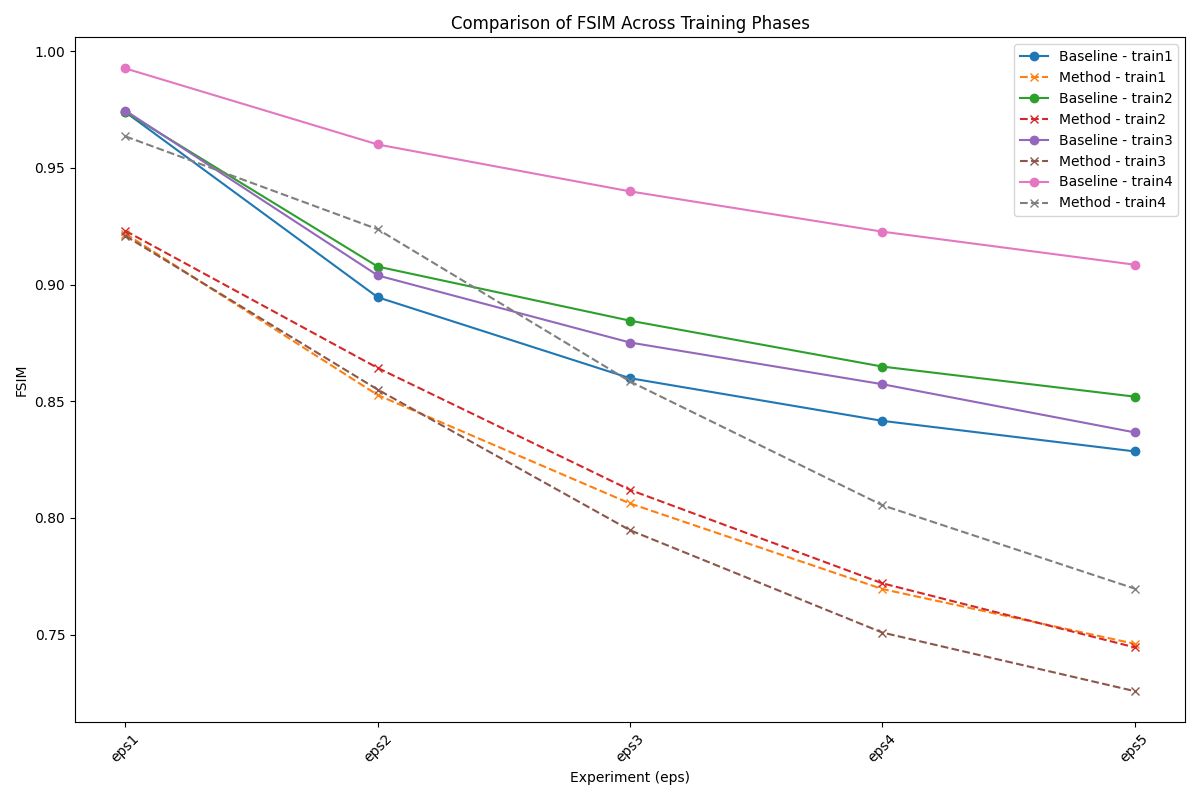
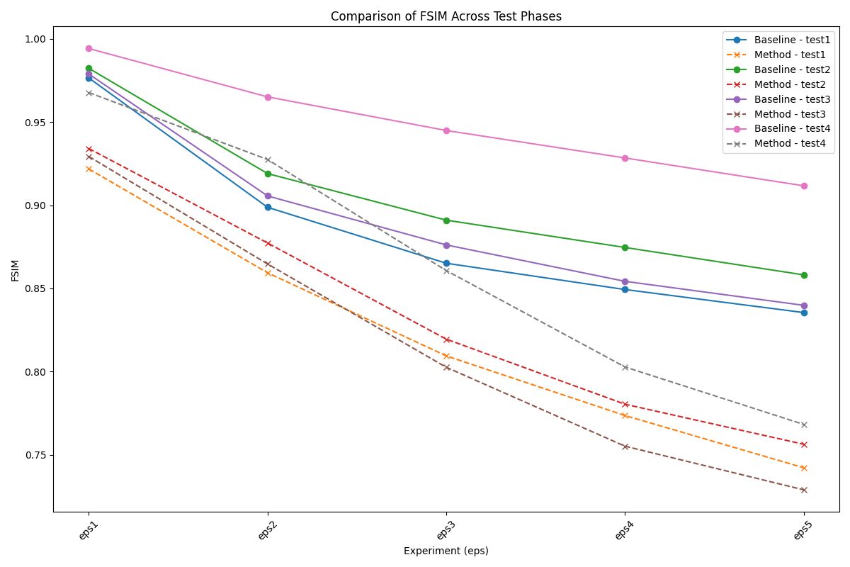
• Feature Similarity Index (FSIM) : Evaluates perceptual similarity by comparing key features such as phase congruency and gradient magnitude between the reference and distorted images.
Experimental Results
| Prompt | Type | SSIM$\uparrow$ (Baseline) | SSIM (Ours) | PSNR$\uparrow$ (Baseline) | PSNR (Ours) | VIFp$\uparrow$ (Baseline) | VIFp (Ours) | FSIM$\uparrow$ (Baseline) | FSIM (Ours) |
|---|---|---|---|---|---|---|---|---|---|
| P1 | Train | 0.6889 | 0.548 | 22.0869 | 18.6758 | 0.1862 | 0.1093 | 0.8285 | 0.7461 |
| Test | 0.6991 | 0.5458 | 22.3317 | 18.4373 | 0.1932 | 0.1087 | 0.8355 | 0.7422 | |
| P2 | Train | 0.7369 | 0.5326 | 23.3199 | 18.8712 | 0.2178 | 0.092 | 0.852 | 0.7446 |
| Test | 0.745 | 0.5433 | 23.4913 | 18.8056 | 0.2251 | 0.0928 | 0.8582 | 0.7563 | |
| P3 | Train | 0.7157 | 0.5168 | 22.3027 | 18.0698 | 0.2081 | 0.1031 | 0.8367 | 0.7258 |
| Test | 0.7241 | 0.5201 | 22.2055 | 17.8572 | 0.2169 | 0.1032 | 0.8399 | 0.7289 | |
| P4 | Train | 0.8181 | 0.5718 | 25.8903 | 19.7084 | 0.29 | 0.1229 | 0.9085 | 0.7697 |
| Test | 0.8249 | 0.5704 | 26.1777 | 19.6394 | 0.2965 | 0.1202 | 0.9117 | 0.7683 |
Our experimental results demonstrate the feasibility of identifying a single adversarial noise pattern that is effective across multiple images. This common noise not only applies successfully to the images it was generated for but also exhibits high transferability to unseen images. Across all evaluation metrics, our approach consistently outperforms the random noise baseline, showcasing its robustness and effectiveness. Notably, in scenarios involving higher epsilon values, the adversarial attack demonstrates remarkable transferability.


Conclusion
SPD-Attack extends the concept of UAPs to adversarial attacks on diffusion-based models and latent space manipulation techniques. By crafting a universal perturbation, it achieves efficient, imperceptible, and generalizable disruptions across tasks, demonstrating significant potential in adversarial robustness research.
Mathematical Notation
| Symbol | Description | Domain/Context |
|---|---|---|
| $x_0$ | Original input data point | Input Space |
| $x_t$ | Data point at diffusion timestep $t$ | Diffusion Process |
| $z_0$ | Latent representation of original input | Latent Space |
| $\mathcal{E}$ | Encoder network | Latent Diffusion Model |
| $\mathcal{D}$ | Decoder network | Latent Diffusion Model |
| $p(x)$ | Data distribution | Probability Distribution |
| $q(x)$ | Empirical data distribution | Probability Distribution |
| $\beta_t$ | Noise variance at timestep $t$ | Diffusion Process |
| $\epsilon_t$ | Random noise added at timestep $t$ | Diffusion Process |
| $\epsilon_{\theta}$ | Noise prediction network | Neural Network |
| $\mu_{\theta}$ | Mean prediction network | Neural Network |
| $\Sigma_{\theta}$ | Variance prediction network | Neural Network |
| $\delta_{adv}$ | Adversarial perturbation | Adversarial Attacks |
| $f_{\theta}$ | Model with parameters $\theta$ | Machine Learning Model |
| $\mathcal{L}$ | Loss function | Optimization |
| $\mathbb{E}$ | Expectation operator | Probability |
| $|\cdot|_p$ | $p$-norm | Norm Calculation |
| $q_{\phi}(z|x)$ | Posterior distribution | Variational Autoencoder |
| $p_{\theta}(z)$ | Prior distribution | Latent Variable Models |
| $D_{KL}$ | Kullback-Leibler Divergence | Information Theory |
| $\mu$ | Mean of a distribution | Statistical Parameter |
| $\sigma^2$ | Variance of a distribution | Statistical Parameter |