Why RoPE Struggles to Maintain Long-Term Decay in Long Sequences?
Rotary Position Embedding (RoPE) improves upon traditional positional encodings but struggles with long-term decay in contexts exceeding its training length, limiting the model's generalization to longer sequences. Our experiments suggest that this issue may stem from a high proportion of obtuse angles on the complex plane between the linear transformations of query and key embeddings.
Why RoPE Struggles to Maintain Long-Term Decay in Long Sequences
Introduction
Rotary Position Embedding (RoPE)
Definition of POCP : POCP specifically measures the angles between each 2D vector component of the query vector \(W_Qx\) and the key vector \(W_Ky\). To compute POCP, the \(d\)-dimensional vectors \(W_Qx\) and \(W_Ky\) are divided into \(\frac{d}{2}\) parts. The angles for each part are calculated, and POCP is the proportion of these angles that exceed 90 degrees:
\[\text{POCP} = \frac{2}{d}\sum_i^{\frac{d}{2}}\textbf{I}(\cos(W_Qx[2i:2i+1], W_Ky[2i:2i+1]) < 0)\]where \(\textbf{I}(A)\) is an indicator function that returns 1 if the event \(A\) occurs, and 0 otherwise.
Experimental Insights: Small POCP Correlates with Better Long-Term Decay in RoPE
A Limitation of RoPE
Without further fine-tuning or the use of interpolation methods
This phenomenon arises from a limitation of RoPE: its inability to maintain long-term decay in significantly longer contexts. The resulting high attention scores on these distant contexts may lead to increased perplexity, impairing the model’s ability to make accurate predictions in these contexts.
A Statistical Analysis of Llama2-7B-4k: As shown in the following figure, we collected \(100\) sequences of \(10,000\) tokens each from Llama2-7B-4k to examine the relationship between the original attention score (\((W_Ky)^TW_Qx\)) and the attention score after applying the RoPE function (\((R(\theta_j)W_Ky)^TR(\theta_i)W_Qx\)), where \(R(\theta_i)\) and \(R(\theta_j)\) denote the RoPE function at position \(i\) and \(j\), respectively.
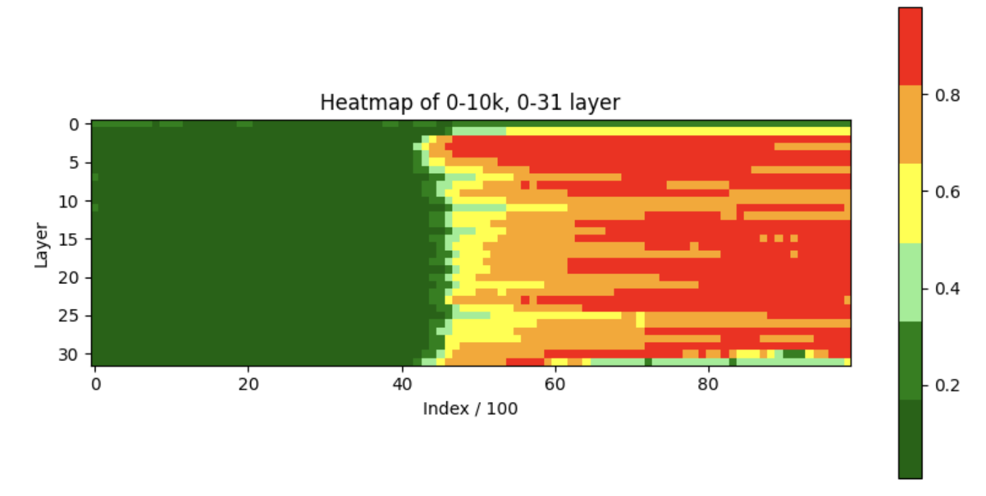
From the statistical analysis, we have observed the following findings::
- After applying the RoPE function, the original attention scores consistently decrease within the trained length but increase beyond it. This suggests that RoPE struggles to maintain long-term decay in significantly extended contexts.
- Within a sequence length of 4k (referring to 4096 tokens), only 20% of the original attention scores exceed the corresponding scores after the application of RoPE.
- For sequences longer than 6000 tokens, 80% of the original attention scores exceed the scores obtained after applying the RoPE function.
To explore the root cause of RoPE’s inability to maintain long-term decay in significantly longer contexts, we investigate the relationship between \(W_Qx\), \(W_Ky\) and the RoPE function in the following sections. Specifically, we examine how \(W_Qx\) and \(W_Ky\) contribute to the high attention scores between \(R(\theta_i)W_Qx\) and \(R(\theta_j)W_Ky\) over long positional distance, where \(R(\theta_i)\) and \(R(\theta_j)\) denote the RoPE function at position \(i\) and \(j\).
Experiments on Randomly Initialized Vectors
We first design a simple experiment on two randomly initialized vectors, denoted as \(\hat{x}\) and \(\hat{y}\):
We test the attention scores between \(R(\theta_i)W_Q\hat{x}\) and \(R(\theta_j)W_K\hat{y}\) (embedding size: \(128\) to \(4096\)) at various positional distances (0 to 16k), conditional on the the Proportion (\(0\%\) to \(100\%\)) of Obtuse angles between \(W_Q\hat{x}\) and \(W_K\hat{y}\) on the Complex Plane (POCP). The code is provided in the Appendix.
As shown in the following figures, we have the following findings:
- Small POCP correlates with better long-term decay in RoPE.
- When the POCP is below \(20\%\) , the attention score between \(W_Qx\) and \(W_Ky\) after applying the RoPE function decreases as the positional distance increases.
- When the POCP exceeds \(50\%\), the attention score between \(W_Qx\) and \(W_Ky\) after applying the RoPE function fluctuates over 4k contexts.
- High-dimensional model embeddings correlate with better long-term decay in RoPE.
- When the embedding size of model is \(128\), as in Llama2-7B, the model can maintain long-term decay if POCP is below \(20\%\). However, with an embedding size of \(4096\), the model can maintain long-term decay if POCP is below \(50\%\). It suggests that a model with a larger embedding size can maintain long-term decay without post-training, leading to better extrapolation ability.
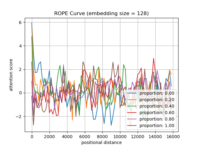
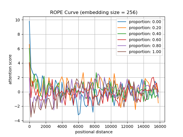
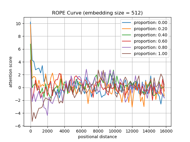
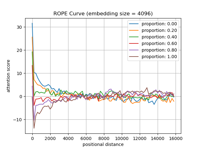
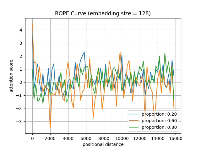
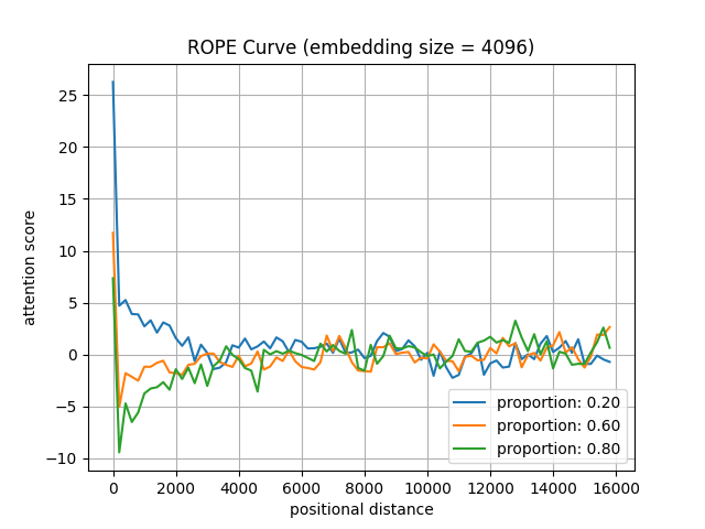
Figure: We test the attention scores between \(W_Qx\) and \(W_Ky\) after applying the RoPE function (embedding size: \(128\) to \(4096\)) at various positional distances (0 to 16k), conditional on the proportion (\(0\%\) to \(100\%\)) of obtuse angles between \(W_Qx\) and \(W_Ky\) on the complex plane.
Experiments in Llama2-7B-4k
Additionally, we argue that embeddings initialized with random weights do not accurately reflect the actual embedding distribution in pre-trained LLMs. Therefore, we select \(W_Qx\) and \(W_Ky\) from first layer of Llama2-7B-4k
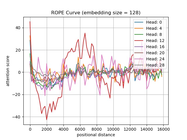
Figure : We randomly select \(W_Q\)x and \(W_Ky\) from the first layer of Llama2-7B-4k.
From the experimental results, we find:
- The attention scores on only a few heads between \(W_Qx\) and \(W_Ky\) after applying the RoPE function are not able to maintain long-term decay in the extended contexts.
- Except for Head-24, the attention score between \(W_Qx\) and \(W_Ky\) after applying the RoPE function generally decreases as the positional distance increases, particularly when the distances range from 0 to 4k.
- Except for Head-12 and Head-24, the attention score between \(W_Qx\) and \(W_Ky\) after applying the RoPE function can slightly fluctuate around 0.
- The attention scores for Head-12 and Head-24 do not maintain long-term decay and fluctuate intensely beyond 4k.
Furthermore, we present the POCP, POCP in the low (last 32 dimensions in the embedding) and high (first 32 dimensions in the embedding) frequency areas, and the original attention score (the attention score between \(W_Qx\) and \(W_Ky\)) in the following table.
| Head | 0 | 4 | 8 | 12 | 16 | 20 | 24 | 28 |
|---|---|---|---|---|---|---|---|---|
| POCP | 0.20 | 0.22 | 0.20 | 0.28 | 0.30 | 0.28 | 0.52 | 0.25 |
| Original attention score | 21 | 30 | 14 | 42 | 8.0 | 7.0 | -3.0 | 17 |
| POCP in low freq (The last 32 dimensions in the embedding.) | 0.25 | 0.13 | 0.44 | 0.25 | 0.50 | 0.63 | 0.50 | 0.13 |
| POCP in high freq (The first 32 dimensions in the embedding.) | 0.13 | 0.31 | 0.06 | 0.38 | 0.19 | 0.06 | 0.56 | 0.38 |
From this table, we find that:
- POCP significantly affects the model’s capacity to maintain long-term decay over extended contexts.
- Except for Head-24, the POCP of all heads is below \(30\%\).
- The POCP of Head-24 exceeds \(50\%\), causing the attention scores between \(W_Qx\) and \(W_Ky\) after applying the RoPE function to fluctuate intensely across the entire 8k range.
- High original attention scores tend to cause intense fluctuations on the extended contexts.
- Although the POCP of Head-12 is only \(28\%\), its original attention score is high among all heads, resulting in more similar angles on the complex plane between \(W_Qx\) and \(W_Ky\). After applying the RoPE function, these similar angles cause the original attention score between each 2D component of \(W_Qx\) and \(W_Ky\) to increase or decrease concurrently, leading to the intense attention score fluctuations beyond 4k.
- There are three heads where the POCP in low frequency area exceeds \(50\%\). Instead, there are only one head where the POCP in high frequency area exceeds \(50\%\).
As a result, we speculate that the heads with high original attention scores and high POCP lead to the increased ppl in the extended contexts.
Comparing POCP Metrics: Llama3-8B-8k vs. Llama3-8B-64k
Finally, we compare POCP between Llama3-8B-8k
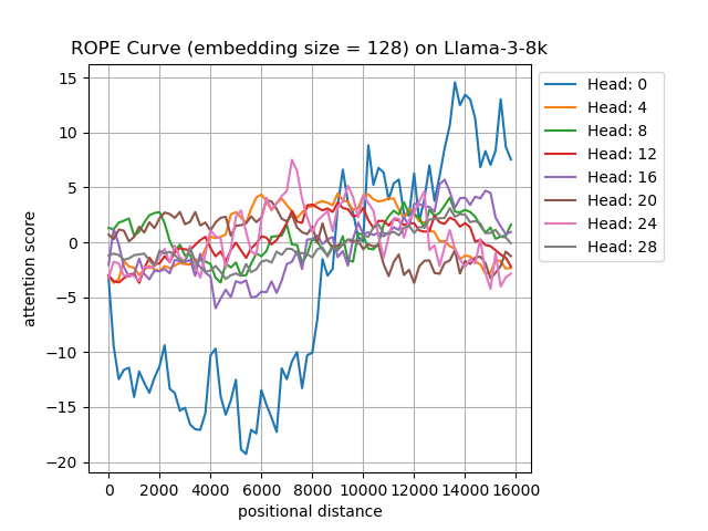
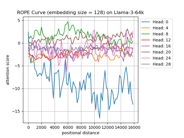
Similarly, we randomly select the \(W_Qx\) and \(W_Ky\) from first layer of Llama3-8B-8k and Llama3-8B-64k to observe the attention score between \(W_Qx\) and \(W_Ky\) after applying the RoPE function with various positional distances (0 to 16k).
| Head | 0 | 4 | 8 | 12 | 16 | 20 | 24 | 28 |
|---|---|---|---|---|---|---|---|---|
| Original attention score | 4.69 | -3.09 | 1.78 | -2.33 | -1.55 | 0.31 | -2.12 | -1.21 |
Figure : We randomly select \(W_Q\)x and \(W_Ky\) from the first layer of Llama3-8B-8k and Llama3-8B-64k.
For Head-0, which has the highest original attention score among all heads, we observe that Llama3-8B-64k maintains long-term decay over a 16k context, whereas Llama3-8B-8k can only do so over an 8k context. For other heads, the attention scores fluctuate around 0 over the entire 16k context. This supports our earlier speculation that high original attention scores tend to cause intense fluctuations on the extended contexts.
Furthermore, we randomly select \(20\) tokens and analyze all \(32\) heads to compare POCP between Llama3-8B-8k and Llama3-8B-64k. Specifically, we use \(10 \times 19 \times 32\) \(W_Qx\) and \(W_Ky\) pairs to calculate POCP for both models and find that:
- The POCP for all token pairs in Llama3-8B-8k is \(0.467\), whereas for Llama3-8B-64k, it is \(0.427\).
- In \(74.6\%\) of token pairs, the POCP in Llama3-8B-8k is higher than in Llama3-8B-64k.
These results demonstrate that POCP significantly influences the model’s ability to maintain long-term decay over long contexts. Additionally, post-training on long contexts primarily decreases the model’s POCP.
Discussion
Are there other factors besides POCP that influence the model’s ability to maintain long-term decay over long contexts?
Aside from POCP, J. Su
To support this findings, we conduct experiments and find that:
- This factor cannot influence the model’s ability to maintain long-term decay over long contexts.
- The magnitude of \(W_K\) in Llama3-8B-8k is lower than that in Llama3-8B-64k.
This suggests that the magnitude of \(W_K\) may be a key factor in influencing the model’s extrapolation ability but does not affect its capacity to maintain long-term decay.
Which role does RoPE play during post-training on long contexts?
Since the RoPE function lacks training parameters, we train the model with long contexts to optimize \(W_Qx\) and \(W_Ky\). Thus, our focus is on how RoPE influences the learning process of \(W_Qx\) and \(W_Ky\). Based on our experiments and related studies, we suppose that RoPE acts as a regularization method, constraining \(W_Qx\) and \(W_Ky\) and their corresponding attention scores during the learning process.
Why the model with RoPE cannot extrapolate directly to longer contexts than those it was trained on?
Recent studies, such as POSE
However, according to J. Su, although the model has encountered these angles during training, it still cannot extrapolate directly to extended contexts. This limitation arises because the model has not been exposed to the attention score distributions in these extended contexts, leading to unseen \(W_Qx\) and \(W_Ky\) in some higher layers. When applied to the RoPE function, these vectors may encounter out-of-distribution issues, potentially resulting in excessively high attention scores on certain tokens in the long distance dependency.
In this blog, we suppose that:
- For directly extrapolating to longer contexts than those it was trained on, the model capture the whole distribution over \(R(\theta_i)W_Qx\) and \(R(\theta_i)W_Ky\) during training.
- To capture the full distribution over \(R(\theta_i)W_Qx\) and \(R(\theta_i)W_Ky\), it is necessary to constrain the representations of \(W_Qx\) and \(W_Ky\) during training. For example, maintaining a small POCP or performing key vector normalization can achieve this.
Future Work
In this blog, we explore a key limitation of RoPE: it cannot maintain long-term decay with significantly longer contexts. This issue may arises from the high POCP. In the future, we will investigate why the model cannot maintain a low POCP on long-context samples and design a new mechanism to address this issue.
Appendix
Here is a code implementation to calculate the POCP, given two randomly initialized vectors:
# Note: This implementation differs from that in Llama2!!!
import torch
import random
import matplotlib.pyplot as plt
from collections import defaultdict

embed_dim = 128

import numpy as np
def normalize(vector):
    norm = np.linalg.norm(vector)
    if norm == 0:
        return vector
    return vector / norm

def softmax(x):
    x = normalize(x)
    e_x = np.exp(x - np.max(x))
    return e_x / e_x.sum(axis=0)

def generate_vectors_with_angle_less_than_90(dim, cent):
    assert dim % 2 == 0, "Embedding dimension must be even."

    # Randomly initialize vectors
    Q = torch.randn(1, dim)
    K = torch.randn(1, dim)

    sub_dim = dim // 2
    for i in range(sub_dim):
        q_sub = Q[0, i*2:(i+1)*2]
        k_sub = K[0, i*2:(i+1)*2]

        # If the dot product of the subcomponents is less than or equal to 0, adjust the subcomponent of K
        while torch.dot(q_sub, k_sub) <= 0:
            K[0, i*2:(i+1)*2] = torch.randn(2)
            k_sub = K[0, i*2:(i+1)*2]

    sample_size = int(sub_dim * cent)
    sample = random.sample(list(range(sub_dim//2, sub_dim)), sample_size//2)
    for i in sample:
        q_sub = Q[0, i*2:(i+1)*2]
        k_sub = K[0, i*2:(i+1)*2]

        # If the dot product of the subcomponents is less than or equal to 0, adjust the subcomponent of K
        while torch.dot(q_sub, k_sub) > 0:
            K[0, i*2:(i+1)*2] = torch.randn(2)
            k_sub = K[0, i*2:(i+1)*2]

    return Q, K

# Define the RoPE function, considering relative position
def apply_rope(tensor, position):
    seq_len, embed_dim = tensor.size()
    print(tensor.shape)
    print(position)
    assert embed_dim % 2 == 0, "Embedding dimension must be even for RoPE."

    half_dim = embed_dim // 2
    freq_seq = torch.arange(half_dim, dtype=torch.float32)
    inv_freq = 1.0 / (10000 ** (freq_seq / half_dim))

    # Calculate sinusoid input
    sinusoid_inp = torch.einsum("i,j->ij", torch.tensor([position], dtype=torch.float32), inv_freq)

    # Calculate sin and cos, and reshape them to match the input tensor's shape
    sin = torch.sin(sinusoid_inp).unsqueeze(0).unsqueeze(0)
    cos = torch.cos(sinusoid_inp).unsqueeze(0).unsqueeze(0)

    # Split the tensor into real and imaginary parts (even and odd indices)
    tensor_1, tensor_2 = tensor[..., 0::2], tensor[..., 1::2]

    # Apply RoPE
    tensor_1_rot = tensor_1 * cos - tensor_2 * sin
    tensor_2_rot = tensor_1 * sin + tensor_2 * cos

    # Interleave the real and imaginary parts back together
    result = torch.zeros_like(tensor)
    result[..., 0::2] = tensor_1_rot
    result[..., 1::2] = tensor_2_rot

    return result

# Apply RoPE, setting the relative position
position_Q = 0  # Position of Q

x = []
dic = defaultdict(list)
for cent in [0.0, 0.2, 0.4, 0.6, 0.8, 1.0]:
    Q, K = generate_vectors_with_angle_less_than_90(embed_dim, cent)
    for position_K in range(0, 16000, 200):
        Q_rope = apply_rope(Q, position_Q)
        K_rope = apply_rope(K, position_K)

        # Calculate Q^T * K
        Q_T = Q_rope.transpose(0, 1)  # Transpose Q
        QK = torch.matmul(K_rope, Q_T) / torch.sqrt(torch.tensor(embed_dim)) # Matrix multiplication

        #print("Position:" + str(position_K) + ", QK^T:", QK)
        item = "proportion: %.2f" % cent
        dic[item].append(QK.item())

for position_K in range(0, 16000, 200):
    x.append(position_K)
for key, val in dic.items():
    #plt.plot(x, softmax(val), linestyle='-', label=key)
    plt.plot(x, val, linestyle='-', label=key)

# Add title and labels
plt.title('ROPE Curve (embedding size = %i)' % embed_dim)
plt.xlabel('positional distance')
plt.ylabel('attention score')

# Display legend
plt.legend(loc=4)

# Show grid lines
plt.grid(True)

# Save the plot to a file
plt.savefig('sample_curve.png')