Restating the Proof of Linear Convergence for Linear GNNs
We lead the readers through the core proof of a pioneering paper that studies the training dynamics of linear GNNs. First, we reorganize the proof and provide a more concise and reader-friendly version, highlighting several key components. In doing so, we identify a hidden error and correct it, demonstrating that it has no impact on the main result. Additionally, we offer a dialectical discussion on the strengths and an overlooked aspect of the approach.
Introduction
(* denotes equal contribution)
In this post, we’re diving into a 2021 paper that attempts to pin down the training dynamics of Graph Neural Networks (GNNs).
This paper
The key idea here is to think of the loss function of a linear GNN as a function over time - during optimization, as time changes, the weights change, and the loss changes accordingly. Here, we imagine each step in the optimization process as moving forward through a tiny time interval. For each discrete time point $t=1,2,…,T$, the gradients for learnable weights to loss decide how the weights would be changed, and thus, further decide how quickly the curve of loss surges up or down at these time points.
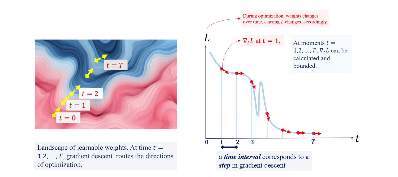
Now, let the time intervals get infinitely closer and closer. Then the discrete optimization process becomes continuous. At any time, correspondingly at any point in the weights’ landscape, how fast the loss changes is determined and bounded by a simple expression.
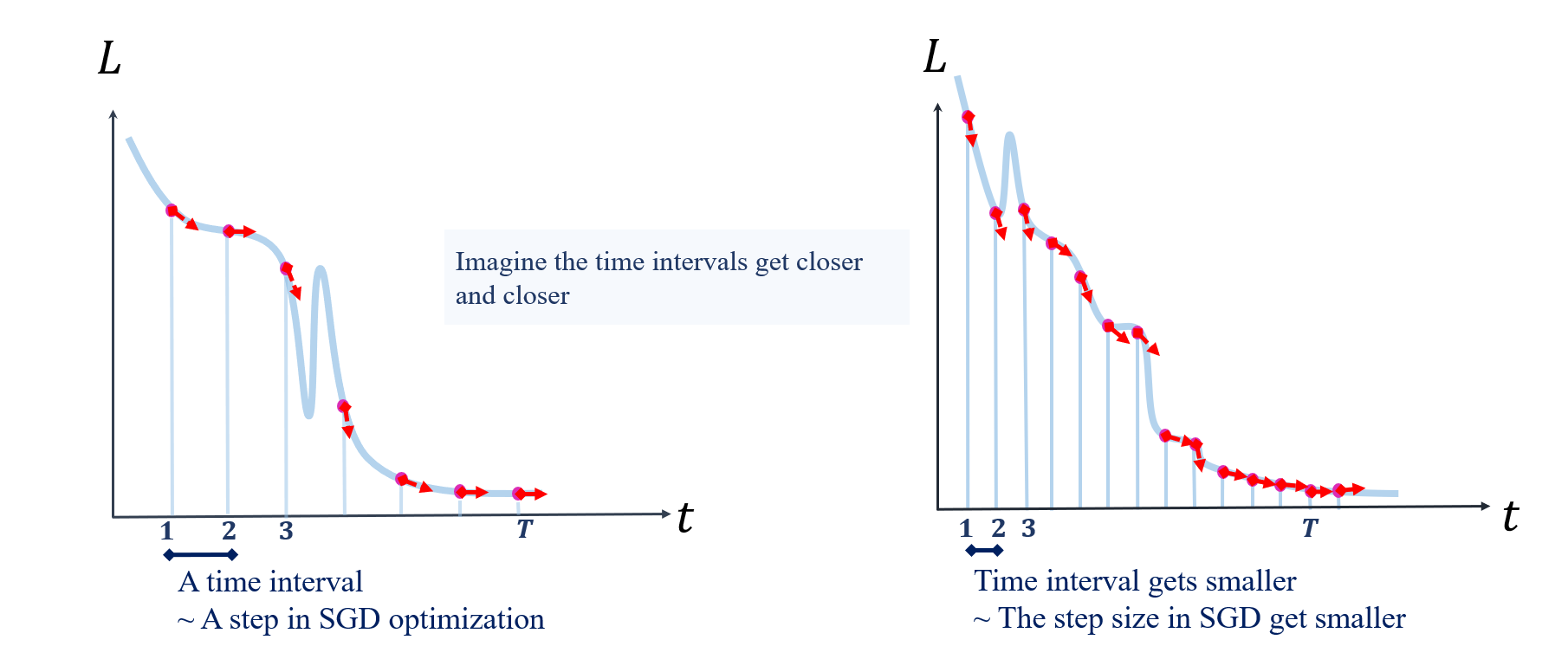
By connecting the dots, now the continuous change in loss can be described by an Ordinary Differential Equation (ODE). With some gradient calculus and simplifications, the result comes down to this beautiful expression:

Surprising
In this blog post, we’ll make the proof flow crystal clear, and also correct that minor hiccup (it won’t take long, promise). Our goal is to make the reasoning behind linear convergence accessible, and bring you more confidence to read and think critically, even if you’re not a math whiz. All you need is a bit of algebra and the chain rule. Ready? Let’s get started!
Minimal Background
In this section, we’ll give you the essential background to grasp the proof of linear convergence for linear GNNs. Don’t be intimidated by the strong conclusion—it’s actually quite accessible with just a bit of background.
We’ll start with the basics of linear GNNs, then move on to some fundamental mathematical tools like matrix gradients and the Kronecker product, which are key to understanding gradient dynamics.
Linear GNNs with Squared Loss
This paper focuses on Linear GNNs, where the non-linear activations are removed, and a simplified squared loss is considered. We’ll assume you’re already familiar with the basic form of GCNs, so let’s dive straight into the formulas below.
\[\begin{eqnarray*} f(X, W, B) &=& W X_{(H)} \\ &=& W B_{(H)} X_{(H-1)} S \\ &=& \cdots \\ &=& W B_{(H)} B_{(H-1)} \cdots B_{(1)} X S^H. \\ \\ L(W, B) &=& \| f(X,W,B)_{*\mathcal{I}} - Y \|_{\mathrm{F}}^2. \end{eqnarray*}\]Note: For detailed explanations on GCN background and the notations, hover here!
In short, the simplest GNN involves just two types of operations: feature propagation over a graph and non-linear transformation, applied alternately. The number of alternations defines how many layers the model has.
In the referenced paper, within this $H$-layer linear GNN $f$ we put below, the initial feature matrix $X$ undergoes propagations through $S$. The intermediate features are transformed by weight matrices $B_1, \ldots, B_H$. Finally, another transformation by $W$ maps the representation of the $H$-th layer into the label space.
Note that the subscript ${ }_{\mathcal{:I}}$ represents indexing, extracting the rows corresponding to the training set nodes. In parallel, $Y$ corresponds to the portion of labels associated with the training nodes.
The above model is trained using gradient descent. To analyze the gradient dynamics, we need a bit of matrix gradient computation.
Matrix Gradients
Here we prepare backgrounds to compute $\nabla_{W}L$ and $\nabla_{B_{\ell}}L, \ell \in [1, H]$, and further, $\nabla_t{L}$. The gradients $\nabla_{W}L$ and $\nabla_{B_{\ell}}L$ determine the direction of change for the current parameters, which in turn influences $\nabla_t{L}$.
- Gradient to linear transformation. Suppose $Y$, $A$ and $B$ to be matrices,
Note: A cautious beginner might ask: why is there a transpose over $B$, but not over $A$? The answer is that, it is due to the layout convention of matrix calculus. The matrix form of multivariable gradients are just a collection of element-wise gradients, and they are organized following different conventions. We refer the reader to the convention sections in wiki page on the Matrix Calculus for about.
- Gradient to least square loss.
-
“Chain rule”. In backpropagation, gradients are passed backward from the output layer down to earlier layers. For example, suppose loss function $L(\cdot)$ to be least square loss, then
\[\hat{Y} = XW \to \nabla_{X}{L} =\nabla_{\hat{Y}}{L} \cdot \nabla_{X}{\hat{Y}} = 2(\hat{Y} - Y)W^{\top}.\]- A subtle but important distinction is that, in matrix calculus, the ‘chain rule’ still applies in an element-wise manner. When these elements are arranged as a matrix and computed collectively, while operations may resemble the chain rule, gradients are not always obtained purely through matrix multiplication along a ‘chain’.
-
For example, let $L: \mathbb{R}^{m \times n} \to \mathbb{R}$ be a function over $\hat{Y}$,
\[\hat{Y} = W_1XW_2 \to \nabla_{X}{L} = W_1^{\top} \nabla_{\hat{Y}}{L} W_2^{\top} .\]
Kronecker Product with Vectorization
When differentiating matrices, we often use the Kronecker product together with the $\mathrm{vec}[\cdot]$ operator.
Note: Hover here
$\mathrm{vec}[\cdot]$ operator. The $\mathrm{vec}[\cdot]$ operator is used to transform a matrix into a vector by stacking its columns on top of one another in a single column vector. For example, if $A$ is an $m \times n$ matrix, $\mathrm{vec}[A]$ rearranges all the columns of $A$ into a vector of size $mn \times 1$. for their basic definitions if you need! We also put an illustrative image here:
Kronecker product. The Kronecker product, denoted by $\otimes$, is an operation on two matrices $A$ and $B$, resulting in a block matrix. Specifically, for an $m \times n$ matrix $A$ and a $p \times q$ matrix $B$, the Kronecker product $A \otimes B$ is an $mp \times nq$ matrix formed by multiplying each element of $A$ by the entire matrix $B$.

-
We’ll frequently encounter the following commonly used expression in the sections ahead.
\[\mathrm{vec}[ABC] = (C^\top \otimes A) \cdot \mathrm{vec}[B]\]- This expression allows us to transform expressions into the more familiar form of matrix-vector multiplication, which can help avoid the complexity of thinking in higher-dimensional spaces.
Proof: Journey to the Theorem
Now that everything is prepared. Let’s dive into the proof! The proof and notations generally follows the original paper.
To make things clearer, in the first place, let’s break this long expression into two parts:
\[f(X, W, B)_{*\mathcal{I}}= \underbrace{\tilde{W}_H}_{W B_{(H)} B_{(H-1)} \cdots B_{(1)}\quad\quad\quad} \underbrace{\tilde{G}_H}_{X (S^H)_{*\mathcal{I}}}.\]This simplifies the loss:
\[L = \| \tilde{W}_H \tilde{G}_H - Y \|_{\mathrm{F}}^2.\]Step 1. Gradients and Optimization Steps.
Note: This part is composed of both the “backward” and “forward” passes. For the backward pass, we derive the gradients of the loss function with respect to the learnable weight matrices. For the forward pass, we derive how much they would shift after a step in the optimization process.
$\tilde{W}_H$, combining all the weight matrices, acts as a “waystation” in both passes. It connects what comes before with what comes next.
It is easy to get $\nabla_{\tilde{W}_H}L = 2(\hat{Y}-Y)\tilde{G}_H^{\top}$.

Now, let’s proceed by deriving gradients for all the learnable weight matrices. The backpropagation process is illustrated in the image below.
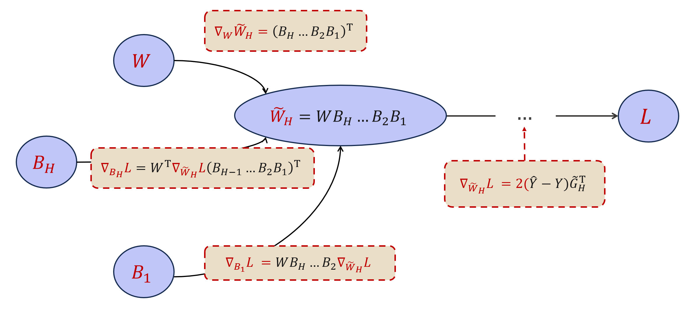
Let’s write out the explict expressions of gradients:
\[\begin{eqnarray} \label{gradients} \begin{aligned} \nabla_{W} L &= \nabla_{\tilde{W}_H} L (B_{(H)} \cdots B_{(1)})^\top, \\ \nabla_{B_{\ell}} L &= (W B_{(H)}\cdots B_{(\ell+1)})^\top \nabla_{\tilde{W}_H} L (B_{(\ell-1)} \cdots B_{(1)})^\top, \ell = 1, \ldots, H. \end{aligned} \end{eqnarray}\]Now we consider the optimization process of this linear model, where $W$ and $B=(B_{(1)},\ldots,B_{(H)})$ are updated via gradient descent:
\[\begin{eqnarray*} \begin{aligned} & W' = W - \alpha \nabla_{W} L, \\ & B'_{(\ell)} = B_{(\ell)} - \alpha \nabla_{B_{(\ell)}} L, \ \ell = 1, \ldots, H. \end{aligned} \end{eqnarray*}\]Once again, we gather at the “waystation node”: how much has $\tilde{W}_H$ shifted?
From here, we’ll write the variables in a vectorized form to pave the way for the following sections. This approach will help us leverage matrix calculus techniques and make the derivations more concise and easier to follow.
\[\begin{eqnarray*} \begin{aligned} & \textrm{vec}[\tilde{W}'_{H}] - \textrm{vec}[\tilde{W}_{H}] \\ = & \textrm{vec}[W' B'_{(H)} \cdots B'_{(1)}] - \textrm{vec}[W B_{(H)} \cdots B_{(1)}] \\ = & \textrm{vec}[(W - \textcolor{blue}{\alpha \nabla_{W} L}) (B_{(H)} - \textcolor{blue}{\alpha \nabla_{B_{(H)}} L}) \cdots (B_{(1)} - \textcolor{blue}{\alpha \nabla_{B_{(1)}} L})] - \textrm{vec}[W B_{(H)} \cdots B_{(1)}] \\ = & - \alpha \underbrace{\textrm{vec}[\textcolor{blue}{\nabla_{W} L} B_{(H)}\cdots B_{(1)}] }_{\textcolor{blue}{\text{part a}}} - \alpha \sum_{\ell=1}^H \underbrace{\textrm{vec}[W B_{(H)}\cdots B_{(\ell+1)} \textcolor{blue}{\nabla_{B_{(\ell)}} L} B_{(\ell-1)} \cdots B_{(1)} ]}_{\textcolor{blue}{\text{part b}}} \\ & + \mathcal{O}(\alpha^2). \end{aligned} \end{eqnarray*}\]This might seem a bit complicated. But when we plug the gradient expressions in Eq.\ref{gradients} and connect the Kronecker product and vectorization
with \(J_{(\ell,H)} := B_{(\ell-1)}\cdots B_{(1)} \otimes (W_{(H)} B_{(H)}\cdots B_{(\ell+1)})^\top, \ \ell = 1, \ldots, H.\)
This symmetry will help us to throw away part b in the next part!
Step 2. The Dynamics.
Note: In this part, we’ll derive the dynamics of $\tilde{W}_H$, and then pass its dynamics to the loss $L$. Following the authors, we throw away the semi-positive term (part b*), reduce all eigenvalues to the minimal, and distinguish the parts of vectors inside and outside the representable space, to derive a bound of the loss dynamics with a favorable form.
- It should be clarified that all the learnable parameters, as well as $\tilde{W}_H$, the loss $L$ and the related eigenvalues and SVD decomposition, is changing over time. We neglect the time notation in this part for simplicity.
Imagine a small step in the optimization as moving forward through a tiny time interval,
we have obtained the dynamics of $\tilde{W}_H$: \(\begin{equation*} \begin{aligned} \frac{\mathrm{d} }{\mathrm{d} t} \mathrm{vec}[\tilde{W}_{H}] :&= \lim_{\alpha \to 0} \frac{\mathrm{vec}[\tilde{W}'_{(H)}] - \mathrm{vec}[\tilde{W}_{(H)}]}{\alpha} \\ &= - \underbrace{[ (B_{(H)}\cdots B_{(1)})^\top (B_{(H)}\cdots B_{(1)}) \otimes I_{m_y}] \mathrm{vec} [\nabla_{\tilde{W}_H}L]}_{\textcolor{blue}{\text{part a'}}} \\ & - \underbrace{\sum_{\ell=1}^H \left( J^\top_{(\ell,H)} J_{(\ell,H)} \right) \mathrm{vec}[\nabla_{\tilde{W}_H} L]}_{\textcolor{blue}{\text{part b'}}}. \\ \end{aligned} \end{equation*}\)
Again, with just one step further from the “waystation” $\tilde{W}_H$, we get the dynamics of $L$:
\[\begin{equation*} \begin{aligned} \frac{\mathrm{d} }{\mathrm{d} t}L = & \frac{\partial L}{\partial \mathrm{vec}[\tilde{W}_H]} \frac{\mathrm{d} }{\mathrm{d} t} \mathrm{vec}[\tilde{W}_H] \\ = & \mathrm{vec} [\nabla_{\tilde{W}_H} L]^\top \frac{\mathrm{d} }{\mathrm{d} t} \mathrm{vec}[\tilde{W}_H] \\ = & - \underbrace{\mathrm{vec} [\nabla_{\tilde{W}_H} L]^\top [ (B_{(H)}\cdots B_{(1)})^\top (B_{(H)}\cdots B_{(1)}) \otimes I_{m_y}] \mathrm{vec} [\nabla_{\tilde{W}_H} L]}_{\textcolor{blue}{\text{part a*}}} \\ & - \underbrace{\sum_{\ell=1}^H \Vert J_{(\ell,H)} \mathrm{vec}[\nabla_{\tilde{W}_H} L] \Vert_2^2}_{\textcolor{blue}{\text{part b*}}} \\ \leq & - \underbrace{\mathrm{vec} [\nabla_{\tilde{W}_H} L]^\top [ (B_{(H)}\cdots B_{(1)})^\top (B_{(H)}\cdots B_{(1)}) \otimes I_{m_y}] \mathrm{vec} [\nabla_{\tilde{W}_H} L]}_{\textcolor{blue}{\text{part a*}}}. \\ \end{aligned} \end{equation*}\]Note: Part b* is dropped!
Denote that
\[\lambda_\mathrm{min} := \text{the minimal eigenvalue of } (B_{(H)}\cdots B_{(1)})^\top (B_{(H)}\cdots B_{(1)}),\]and plug $\nabla_{\tilde{W}_H} L=2(\hat{Y}-Y)\tilde{G}_H^{\top}$ into the expression above, we have
\[\begin{eqnarray} \label{dynamics} \begin{aligned} \frac{\mathrm{d} }{\mathrm{d} t}L \leq & - \lambda_{\rm min}\cdot \Vert \mathrm{vec} [\nabla_{\tilde{W}_H} L] \Vert^2_2 \\ = & - 4\lambda_{\rm min}\cdot((\tilde{G}_H \otimes I_{m_y})\mathrm{vec} [\hat{Y}-Y])^\top ((\tilde{G}_H \otimes I_{m_y})\mathrm{vec} [\hat{Y}-Y]) \\ = & - 4\lambda_{\rm min}\cdot \textcolor{blue}{\underbrace{\mathrm{vec}[\hat{Y}-Y]^\top \left[ \tilde{G}^\top_H \otimes I_{m_y} \right] \left[ \tilde{G}_H \otimes I_{m_y} \right] \mathrm{vec}[\hat{Y}-Y]}_{\textrm{Eq.(*)}}}. \end{aligned} \end{eqnarray}\]Next, let’s bound Eq.(*).
Before bounding Eq.(*), we introduce the notation $\mathbf{P}$, which projects vectors onto the column space of \(\tilde{G}_H^{\top} \otimes I_{m_y}\).
Denote the SVD decomposition of \(\tilde{G}_H^{\top} \otimes I_{m_y}\) to be \(U \Sigma V^{\top}\), then \(\mathbf{P}=U U^{\top}\).
\[\begin{equation*} \begin{aligned} \textcolor{blue}{\textrm{Eq.(*)}} &= \mathrm{vec}[\hat{Y}-Y]^{\top} U (\Sigma)^2 U^{\top} \mathrm{vec}[\hat{Y}-Y] & \textcolor{gray}{\text{(SVD of $\tilde{G}_H^{\top} \otimes I_{m_y}$)}} \\ & \geq \sigma_{\mathrm{min}}^2(\tilde{G}_H) \cdot \mathrm{vec}[\hat{Y}-Y]^{\top} U U^{\top} \mathrm{vec}[\hat{Y}-Y] & \textcolor{gray}{\text{($\sigma_{\mathrm{min}}(\tilde{G}_H) := \sigma_{\mathrm{min}}(\tilde{G}_H\otimes I_{m_y})$)} } \\ & \geq \sigma_{\mathrm{min}}^2(\tilde{G}_H) \cdot \Vert \mathbf{P} \mathrm{vec}[\hat{Y}-Y]\Vert_2^2 & \textcolor{gray}{\text{(Projector to the column space)}} \end{aligned} \end{equation*}\]Now, we split \(\mathrm{vec}[\hat{Y}-Y]\) into two parts:
\[\mathrm{vec}[\hat{Y}-Y] = \underbrace{\mathrm{vec}[Y^*-Y]}_{\text{orthogonal to [$\tilde{G}_H^{\top} \otimes I_{m_y}$]}} - \underbrace{\mathrm{vec}[Y^*-\hat{Y}]}_{\text{resides in [$\tilde{G}_H^{\top} \otimes I_{m_y}$]}}.\]Thus we have
\[\begin{equation*} \begin{aligned} \textcolor{blue}{\text{Eq.(*)}} &\geq \sigma_{\mathrm{min}}^2(\tilde{G}_H) \cdot \Vert \mathrm{vec}[Y^* - \hat{Y}]\Vert_2^2 \\&= \sigma_{\mathrm{min}}^2(\tilde{G}_H) (\Vert \mathrm{vec}[\hat{Y}-Y]\Vert_2^2 - \Vert \mathrm{vec}[Y^* - Y]\Vert_2^2 ) \\&= \sigma_{\mathrm{min}}^2(\tilde{G}_H) (L - L^*_H). \end{aligned} \end{equation*}\]where $L^*_H$ stands for the optimal loss for this $H$-layer linear GNN.
Combining the derivation to $L$, Eq.(\ref{dynamics}) comes into:
\[\begin{equation} \label{L_grad} \frac{\mathrm{d}}{\mathrm{d} t}L \leq - 4\lambda_{\rm min}\sigma^2_{\rm min}(\tilde{G}_H) (L - L^*_H). \end{equation}\]Step 3. Solving the ODE.
Note: ODE is always used to describe and solve the dynamics of a system. Now, we are just one step away from the final result.
Having Eq.(\ref{L_grad}), and use the fact that $\frac{\mathrm{d} }{\mathrm{d} t}L^*_H = 0$, we have
\[\begin{equation*} \frac{\mathrm{d}}{\mathrm{d} t}(L- L^*_H) \leq - 4\lambda_{\rm min}\sigma^2_{\rm min}(\tilde{G}_H) (L - L^*_H). \end{equation*}\]Solving this ODE we have
\[\begin{equation*} \begin{aligned} L_T - L^*_H & \leq (L_0 - L^*_H) e^{-4\sigma^2_{\rm min}(\tilde{G}_H) \int_{0}^T \lambda_{\rm min,t}} & \\ & \leq (L_0 - L^*_H) e^{-4 \lambda^{(H)}_T \sigma^2_{\rm min}(\tilde{G}_H) T} \\ & = (L_0 - L^*_H) e^{-4 \lambda^{(H)}_T \sigma^2_{\rm min}(X (S^H)_{*\mathcal{I}}) T}, & \end{aligned} \end{equation*}\]where \(\lambda^{(H)}_T := {\rm inf}_{t \in [0,T]} {\lambda_{\rm min}((B_{(H),t}\cdots B_{(1),t})^\top (B_{(H),t}\cdots B_{(1),t})) }\).
This finishes the proof.
A Minor Mistake in the Original Paper
The error exits in the following equation, which appear in Appendix A.1.3, the last inequality in Page 18 of the original paper. It writes:
\[\begin{equation*} \begin{aligned} & \left( \Vert \mathrm{vec}[\hat{Y}-Y] \Vert_2 - \Vert (I_{m_y n} - \mathbf{P}_{\tilde{G}_H^\top \otimes I_{m_y}}) \mathrm{vec}[Y] \Vert_2 \right)^2 \\ \geq & \Vert \mathrm{vec}[\hat{Y}-Y] \Vert^2_2 - \Vert (I_{m_y n} - \mathbf{P}_{\tilde{G}_H^\top \otimes I_{m_y}}) \mathrm{vec}[Y] \Vert^2_2, \end{aligned} \end{equation*}\]where our notation \(\mathbf{P}\) matches \(\mathbf{P}_{\tilde{G}_H^\top \otimes I_{m_y}}\) here for neatness.
By simple calculation, one can verify that the inequality only holds when
\[\begin{equation*} \underbrace{\Vert (I_{m_y n} - \mathbf{P}_{\tilde{G}_H^\top \otimes I_{m_y}}) \textrm{vec}[Y] \Vert_2}_{L_{H}^{*}} \geq \underbrace{\Vert \textrm{vec}[\hat{Y}-Y] \Vert_2}_{L}, \end{equation*}\]which is contrary to the fact that $L^*_H \leq L$.
Critical Thinking
We love to make the theorem in the introduced paper clear and engaging. Now, let’s dive into the chaos — think a bit deeper, and question what really matters.
Note: In this part, we remind readers that the continuous time perspective is an approximation. However, the inherent errors are often overlooked, leading to potentially overconfident conclusions. Nonetheless, on the other hand, treating discrete events as continuous has proven effective, not only in neural network analysis but also in various other scientific fields. We believe this approach is valuable, as long as we remain mindful of its limitations and recognize what has truly been achieved.
The Overlooked Gap.
The paper we’re talking about makes a bold claim. But does it always hold up in practice? Do real GNNs (when framed as a regression problem) truly guarantee convergence?
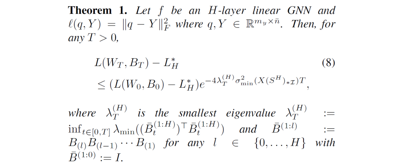
Some gaps are pretty obvious, and the authors
Dynamics at Discrete Moments.
Take another look at these two diagrams I drew earlier:
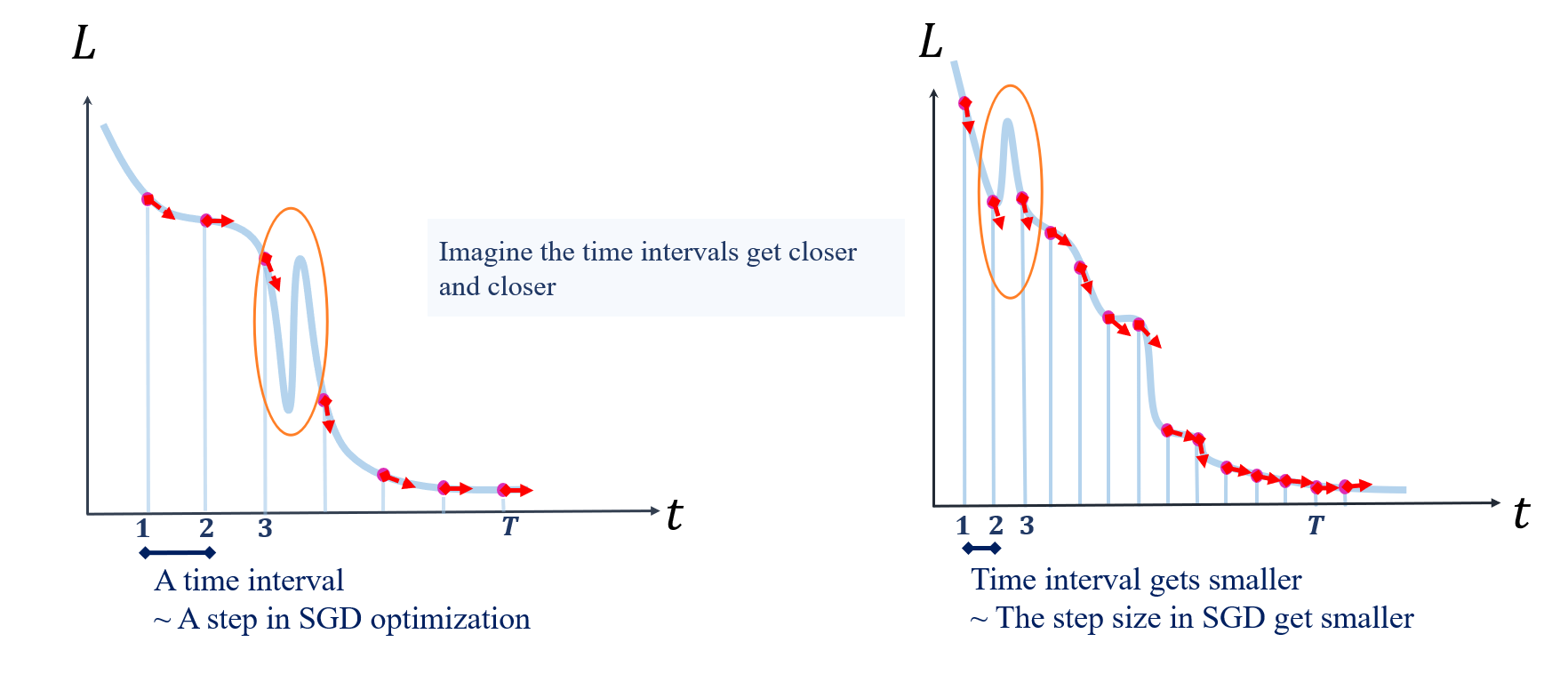
When I drew the illustration, I was thinking about the dynamics we’re trying to capture. So at each time point, I make the loss surge downward, showing that $\nabla_{t} L$ is “under control” (meets Eq.(\ref{L_grad})) at these points, because at these moments, we are adjusting weight matrices using principles based on their current gradients. However, we can only control things at these specific moments. So besides these time points, I drew sharp upward surges, as highlighted by the orange circles.
In the introduction, we hinted at the intuition behind gradient dynamics:
“The loss is like a light particle swimming through a velocity field; how fast it surges is controlled by the field anywhere as it swims.”
But in reality, “anywhere” is impossible, no matter how much we reduce the step size. The actual process is more like a particle speeding out at an initial velocity, maintaining that speed until landing at a new point, and then immediately flying to the next point with a new velocity. Thus, the trajectories solved by ODEs and the actual loss trajectories only share the same slopes at discrete points.
A Balanced View.
The paper’s claim might be a bit too confident. But pointing out these issues doesn’t mean we’re against using dynamic gradients. Our main point is that we need to know what’s uncertain.
The limitation of this approach was pointed out by an anonymous reviewer of the early paper
“I appreciate the attempt to make the analysis more rigorous in terms of ‘learning speed’. Although perhaps a better way to work out a realistic lambda would be to bound the error one gets by taking the continuous time approximation of the original difference equations and choose lambda based on when this error can be argued to have a negligible effect … there is no guarantee that this will imply a reasonable correspondence between the discrete and continuous time versions, where mere stability isn’t enough.” –Reviewer 733d
Even so, the method that study the discrete optimization process from a continuous viewpoint is widely adopted
What’s more, we notice that similar approaches, which treat inherently discrete entities as continuous by using an ODE or PDE to model the process, are also widely adopted in many other scientific areas. For example, when establishing mathematical models of epidemic diseases, researchers treat the disease spreading process among people as a continuous flow, which has led to many valuable insights. We refer the readers to the SI and SIS models introduced HERE on Albert-László Barabási’s website.
Therefore, we need to recognize both sides of the coin: such methods that convert discrete processes into continuous ones are widely applied and proven effective. While acknowledging their utility, we must also be aware of what we truly understand. It’s not just about “whether there’s a gap” — it’s about “whether we recognize it and are willing to accept it”.
Conclusion
In this blog post, we introduce an important theorem in the field of GNN optimization using vivid language and illustrations. Our flow builds upon the original paper’s proof strategy, with a clear yet detailed background provided. For the proof, we offer intuitive explanations and concise steps, making it easier for readers to follow. We also point out a small error in the original proof.
We believe that the methodology of this paper can not only help in understanding the optimization of GNNs, but may also be applicable to other architectures that share some similarities, such as SSMs (State Space Models). And our post would lead more researchers to engage in the topics.
One of the advantages of writing in blog format is that we can discuss related ideas more comprehensively. For instance, we acknowledge the strengths of the paper while also discussing, in a balanced manner, the overlooked aspects of the gradient dynamics method. By incorporating discussions from both inside and outside the neural network field, we help readers understand why this issue exists and why it has been overlooked to some extent.
Thanks for reading! We hope you enjoyed this post and found it helpful.