Intricacies of Feature Geometry in Large Language Models
Studying the geometry of a language model's embedding space is an important and challenging task because of the various ways concepts can be represented, extracted, and used. Specifically, we want a framework that unifies both measurement (of how well a latent explains a feature/concept) and causal intervention (how well it can be used to control/steer the model). We discuss several challenges with using some recent approaches to study the geometry of categorical and hierarchical concepts in large language models (LLMs) and both theoretically and empirically justify our main takeaway, which is that their orthogonality and polytopes results are trivially true in high-dimensional spaces, and can be observed even in settings where they should not occur.
An Overview of the Feature Geometry Papers
We present several ablation results and theoretical arguments highlighting challenges with the theses of two recent works, the ICML 2024 Mechanistic Interpretability Workshop 1st prize winning paper - The Geometry of Categorical and Hierarchical Concepts in LLMs
The methodology described in the two papers we study is as follows – they split the computation of a large language model (LLM) into everything before the unembedding and the unembedding itself:
\[P(y \mid x) = \frac{\exp(\lambda(x)^\top \gamma(y))}{\sum_{y' \in \text{Vocab}} \exp(\lambda(x)^\top \gamma(y'))}\]where:
- $\lambda(x)$ is the context embedding for input $x$ (last token’s residual after the last layer)
- $\gamma(y)$ is the unembedding vector for output $y$ (using the unembedding matrix $W_U$)
They formalize a notion of a binary concept as a latent variable $W$ that is caused by the context $X$ and causes output $Y(W=w)$ depending only on the value of $w \in W$.
Comment: Crucially, this restricts their methodology to only work with concepts that can be differentiated by single-token counterfactual pairs of outputs. For instance, it is not clear how to define several important concepts such as “sycophancy” and “truthfulness” using their formalism.
They then define linear representations of a concept in both the embedding and unembedding spaces:
In the unembedding space, $\barγ_W$ is considered a representation of a concept W if \(\gamma (Y (1)) − \gamma (Y (0)) = \alpha\bar \gamma_W\) almost surely, where $\alpha > 0$.
Comment: This definition has the hidden assumption that each pair $(Y(0), Y(1))$ sampled from the vocabulary would only correspond to a unique concept. For instance, (“king”, “queen”) can correspond to a variety of concepts such as “male ⇒ female”, “k-words ⇒ q-words”, and “n’th card ⇒ (n-1)’th card” in a deck of playing cards.
In the embedding space, they say that $\bar{\lambda}_W$ is a representation of a concept $W$ if we have $\lambda_1 - \lambda_0 \in \text{Cone}(\bar{\lambda}_W)$ for any context embeddings $\lambda_0, \lambda_1 \in \Lambda$ that satisfy \(\frac{\mathbb{P}(W = 1 \mid \lambda_1)}{\mathbb{P}(W = 1 \mid \lambda_0)} > 1 \quad \text{and} \quad \frac{\mathbb{P}(W, Z \mid \lambda_1)}{\mathbb{P}(W, Z \mid \lambda_0)} = \frac{\mathbb{P}(W \mid \lambda_1)}{\mathbb{P}(W \mid \lambda_0)},\) for each concept $Z$ that is causally separable with $W$. The first condition means that the probability of a concept $W$ being true given a context embedding $\lambda_1$ is greater than under context embedding $\lambda_0$.
Now, in order to work with concept representations (i.e. look at similarities, projections, etc.), we need to define an inner product. They provide the following definition
$\textbf{Definition 3.1 (Causal Inner Product).}$ A $\textit{causal inner product}$ $\langle \cdot, \cdot \rangle_\mathcal{C}$ on $\overline{\Gamma} \simeq \mathbb{R}^d$ is an inner product such that \(\langle \overline{\gamma}_W, \overline{\gamma}_Z \rangle_\mathcal{C} = 0,\) for any pair of causally separable concepts $W$ and $Z$.
Comment: Note that this definition allows the inner product $<a,b>=0 \forall (a,b) : a\ne b$ to be a causal inner product. As we show, the whitening transformation they apply as an explicit example of a causal inner product does indeed make almost everything almost orthogonal.
This choice turns out to have the key property that it unifies the unembedding and embedding representations
$\text{Theorem 3.2 (Unification of Representations).}$ Suppose that, for any concept $W$, there exist concepts \(\{ Z_i \} _{i=1}^{d-1}\) such that each \(Z_i\) is causally separable with \(W\) and \(\{ \overline{\gamma}_W \} \cup \{ \overline{\gamma}_{Z_i} \}_{i=1}^{d-1}\) is a basis of \(\mathbb{R}^d\). If \(\langle \cdot, \cdot \rangle_\mathcal{C}\) is a causal inner product, then the Riesz isomorphism \(\overline{\gamma} \mapsto \langle \overline{\gamma}, \cdot \rangle_\mathcal{C}\), for \(\overline{\gamma} \in \overline{\Gamma}\), maps the unembedding representation \(\overline{\gamma}_W\) of each concept \(W\) to its embedding representation \(\overline{\lambda}_W\):
\[\langle \overline{\gamma}_W, \cdot \rangle_\mathcal{C} = \overline{\lambda}_W^\top.\]For an explicit example of a causal inner product, they consider the whitening transformation using the covariance matrix of the unembedding vectors as follows
where $\gamma$ is the unembedding vector, $\mathbb{E}[\gamma]$ is the expected unembedding vector, and $\text{Cov}$ is the covariance matrix of $\gamma$. They show that under this transformation, the embedding and unembedding representations are the same.
Now, for any concept $W$, its vector representation $\ell_W$ is defined to be:
\[\bar{\ell}_w = (\tilde{g}_w^\top\mathbb{E}(g_w)) \tilde{g}_w, \text{where} \,\,\,\, \tilde{g}_w = \frac{\text{Cov}(g_w)^\dagger\mathbb{E}(g_w)}{\|\text{Cov}(g_w)^\dagger\mathbb{E}(g_w)\|_2}\]These are their main orthogonality results
$\textbf{Theorem 8 (Hierarchical Orthogonality).}$ Suppose there exist such vector representations $l_w$ for binary concepts (where $\ell_{w_1} - \ell_{w_0}$ is the linear representation of $w_0 \Rightarrow w_1$), the following orthogonality relations hold:
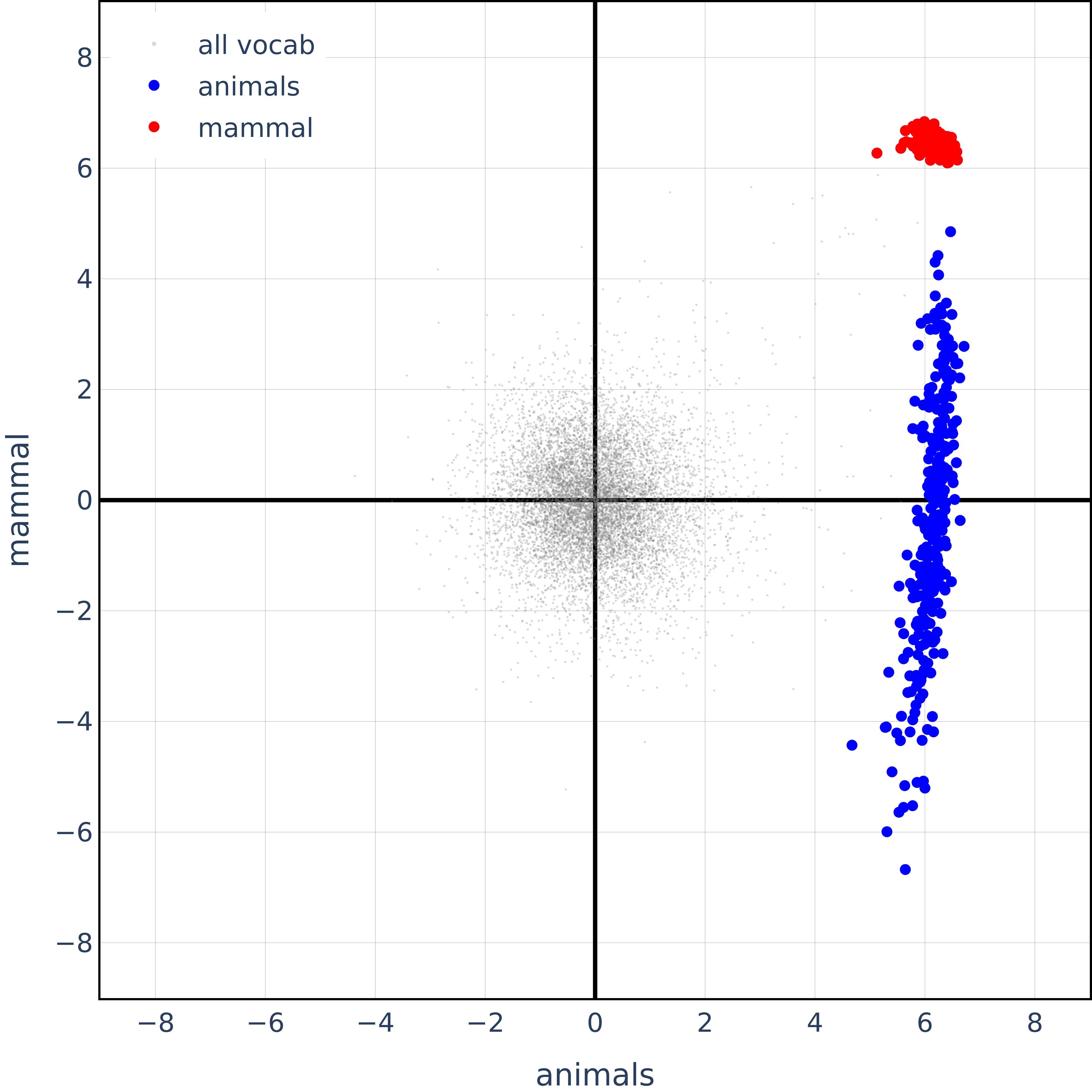
\[\ell_w \perp (\ell_z - \ell_w) \quad \text{for } z \prec w\]\[\ell_w \perp (\ell_{z_1} - \ell_{z_0}) \quad \text{for } \{z_0, z_1\} \prec w\]Comment: This illustrates that for hierarchical concepts mammal $\prec$ animal, we have $\ell_{animal} \perp (\ell_{mammal} - \ell_{animal})$. They prove this holds true and empirically validate it by plotting various animal representation points in the 2D span of the vectors for animal and mammal.
\[(\ell_{w_1} - \ell_{w_0}) \perp (\ell_{z_1} - \ell_{z_0}) \quad \text{for } \{z_0, z_1\} \prec \{w_0, w_1\}\] \[(\ell_{w_1} - \ell_{w_0}) \perp (\ell_{w_2} - \ell_{w_1}) \quad \text{for } w_2 \prec w_1 \prec w_0\]Similarly, this means $\ell_{animal} \perp (\ell_{mammal} - \ell_{reptile})$.
Lastly, they show that in their transformed space, categorical features form polytopes in $n$-dimensions. They empirically show these results to hold in the Gemma-2B model and use the WordNet hierarchy to validate them at scale.
Ablations
While we find the dataset they study (animal categories and hierarchies) to indeed exhibit the geometry they predict, to study concepts that do not form such semantic categories and hierarchies, we add the following two datasets:
Semantically Correlated Concepts
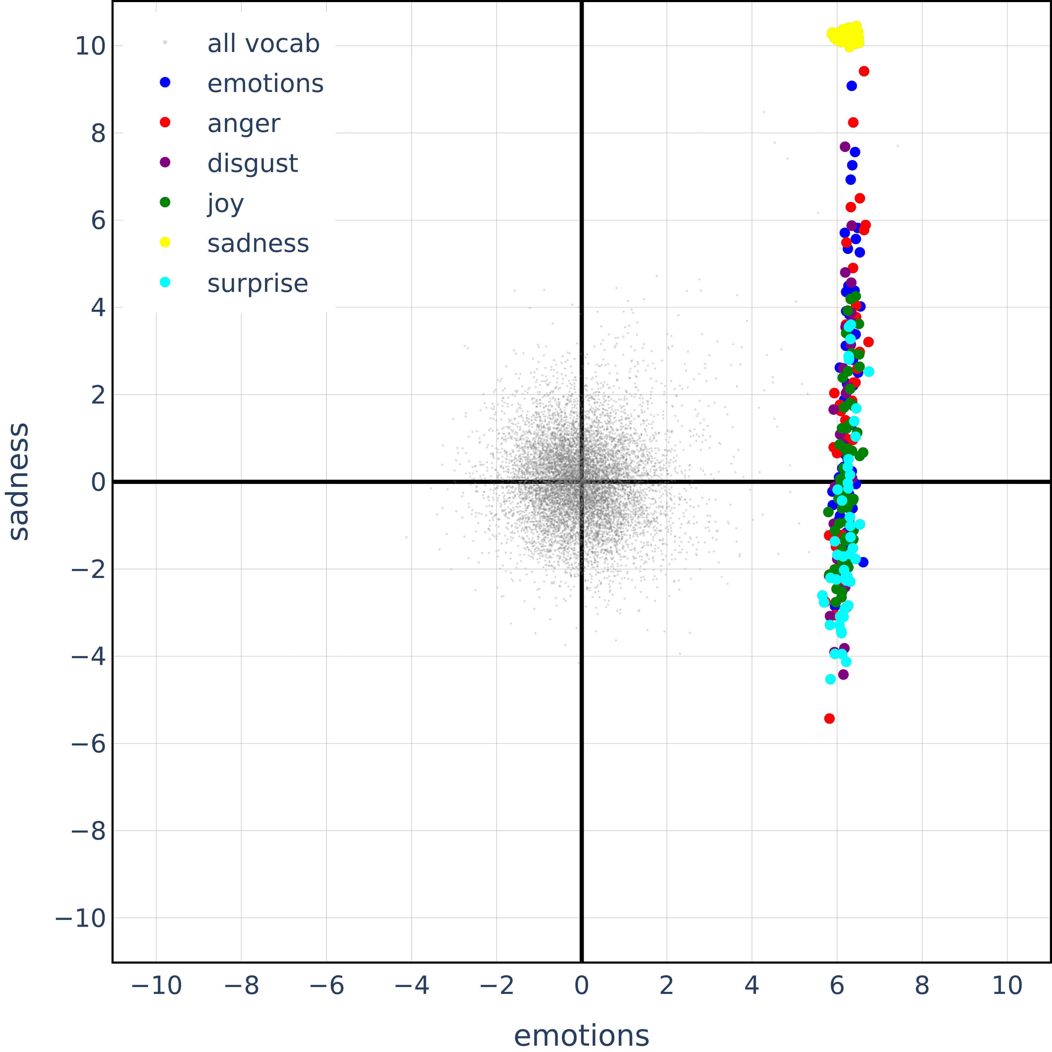
First, an “emotions” dictionary for various kinds of emotions split in various top-level emotions. Note that these categories are not expected to be orthogonal (for instance, joy and sadness should be anti-correlated). We create this via a simple call to ChatGPT:
1
2
3
4
5
6
7
8
 emotions = {
   'joy': ['mirth', 'thrill', 'bliss', 'relief', 'admiration', ...],
   'sadness': ['dejection', 'anguish', 'nostalgia', 'melancholy', ...],
   'anger': ['displeasure', 'spite', 'irritation', 'disdain', ...],
   'fear': ['nervousness', 'paranoia', 'discomfort', 'helplessness', ...],
   'surprise': ['enthrallment', 'unexpectedness', 'revitalization', ...],
   'disgust': ['detestation', 'displeasure', 'prudishness', 'disdain', ...]
}
Random Nonsensical Concepts
Next, we add a “nonsense” dataset that has five completely random categories where each category is defined by several (order of 100) completely random objects completely unrelated to the top-level categories:
1
2
3
4
5
6
7
 nonsense = {
   "random 1": ["toaster", "penguin", "jelly", "cactus", "submarine", ...],
   "random 2": ["sandwich", "yo-yo", "plank", "rainbow", "monocle", ...],
   "random 3": ["kiwi", "tornado", "chopstick", "helicopter", "sunflower", ...],
   "random 4": ["ocean", "microscope", "tiger", "pasta", "umbrella", ...],
   "random 5": ["banjo", "skyscraper", "avocado", "sphinx", "teacup", ...]
}
Please see the reproducibility statement in the end for the exact details of our setup and the full dictionaries.
Hierarchical features are orthogonal - but so are semantic opposites!?
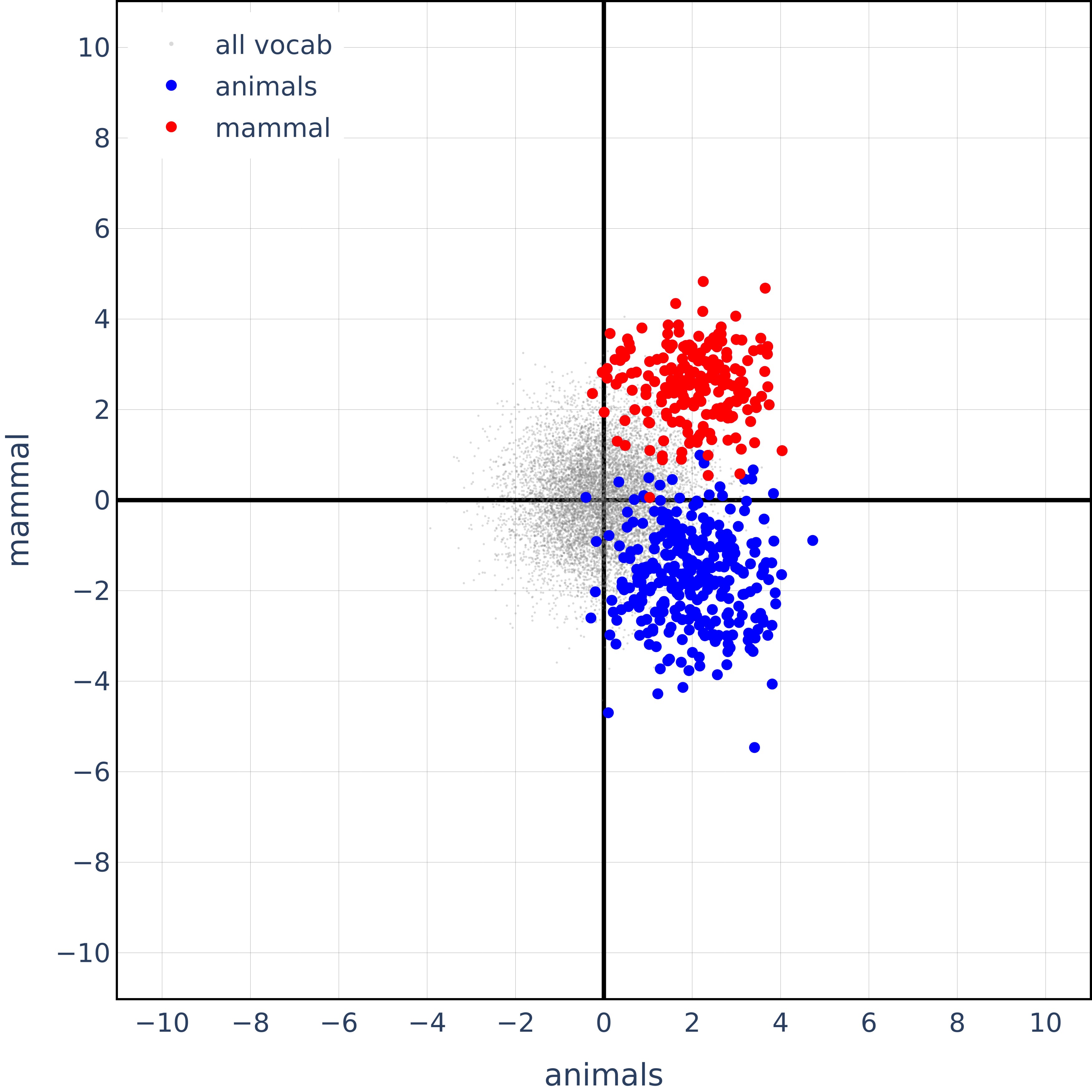
Now, let’s look at their main experimental results for animal hierarchies (see Fig. 2 in their original paper):
And this is the first ablation we run – all emotion words in the 2D span of sadness and emotions:
Specifically, this is what we get for joy vectors in the span of sadness. Note that the orthogonality observed is very similar to that in the case of animal hierarchies.
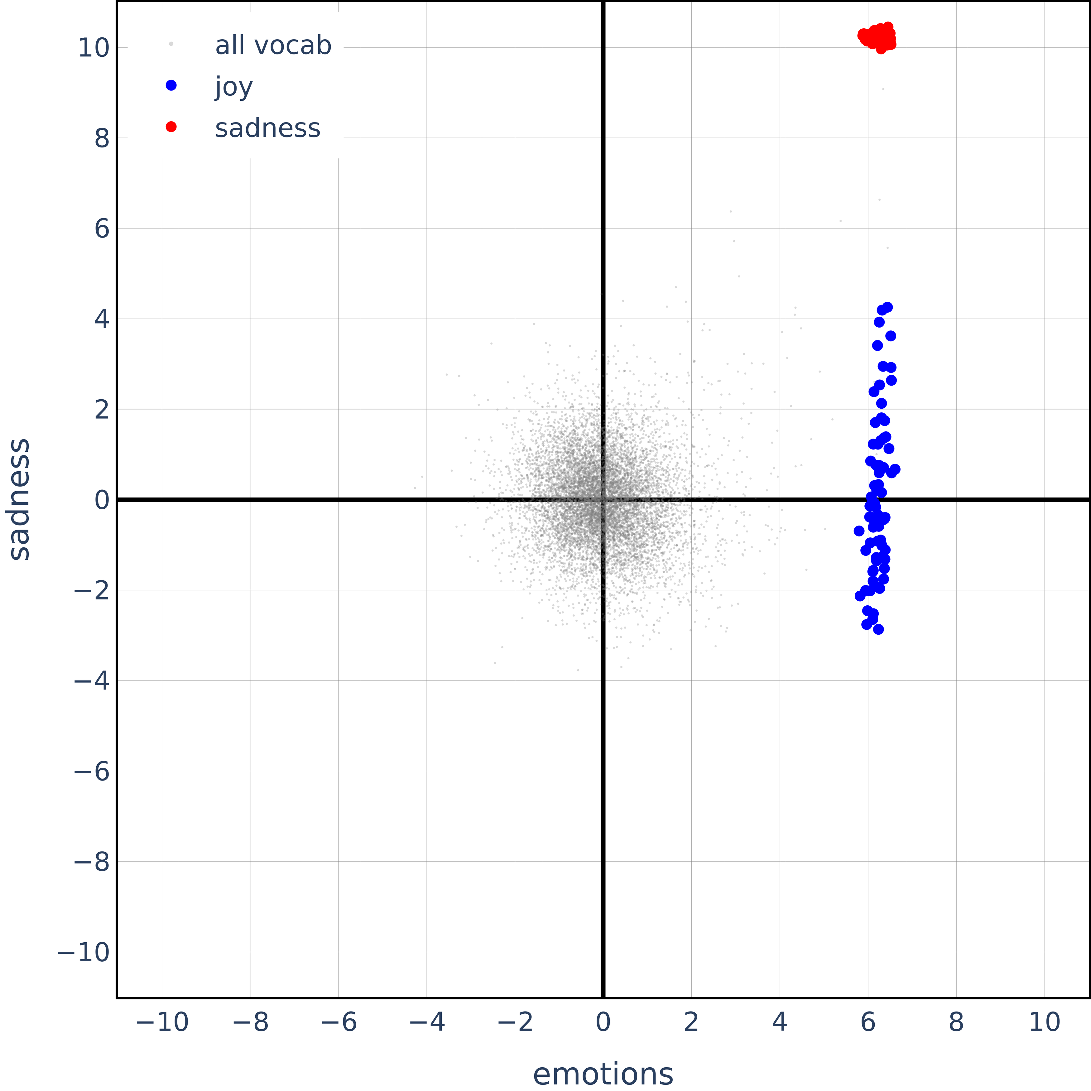
Should we really have joy so un-correlated with sadness? Sadness and joy are semantic opposites, so one should expect the vectors to be anti-correlated rather than orthogonal.
Also, here’s the same plot but for completely random, non-sensical concepts:
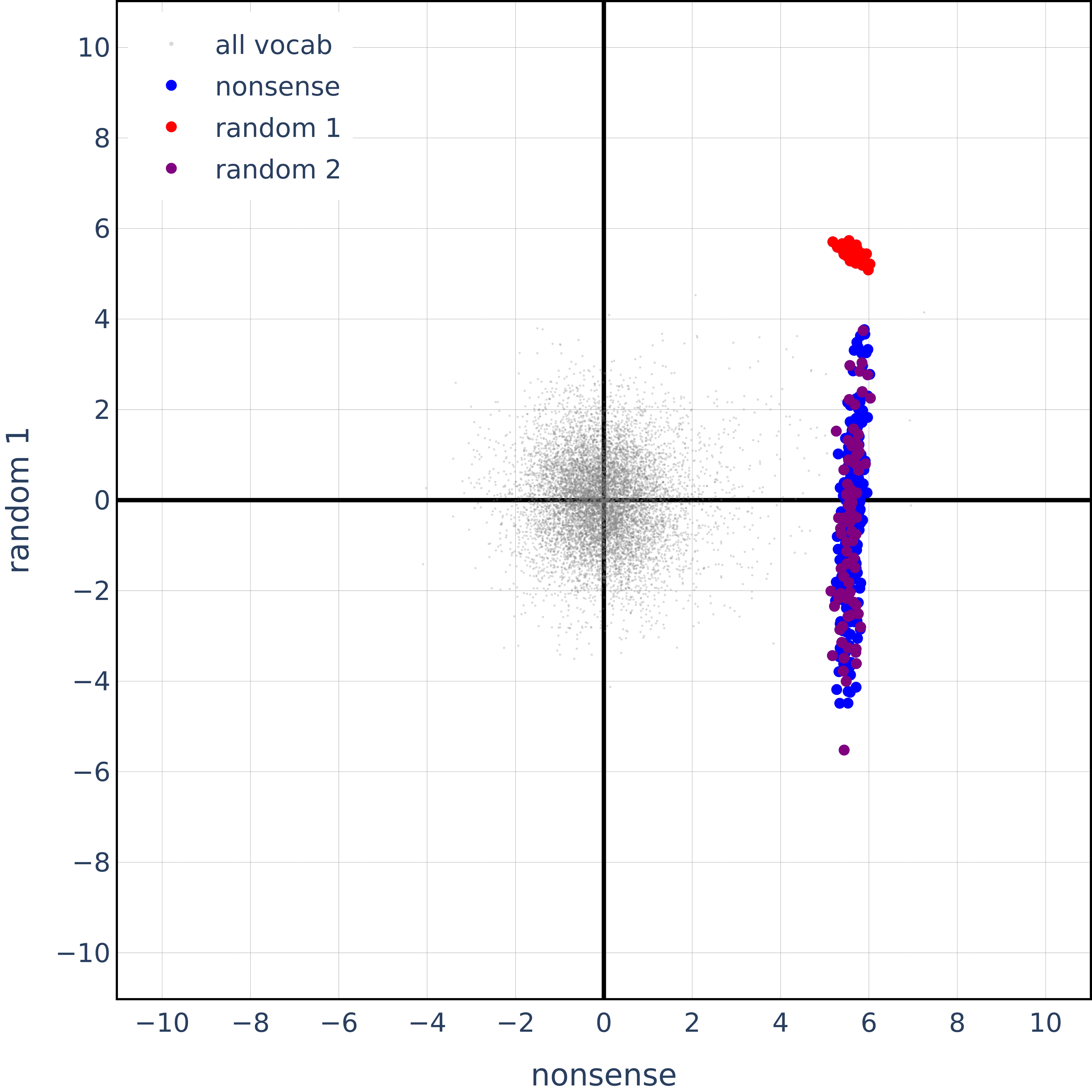
It seems like their orthogonality results, while true for hierarchical concepts, are also true for semantically opposite concepts and totally random concepts. In the next section, we will show theoretically that in high-dimensions, random vectors, and in particular those obtained after the whitening transformation, are expected to be trivially orthogonal with a very high probability.
Categorical features form simplices - but so do totally random ones!?
Here is the simplex they find animal categories to form (see Fig. 3 in their original paper):
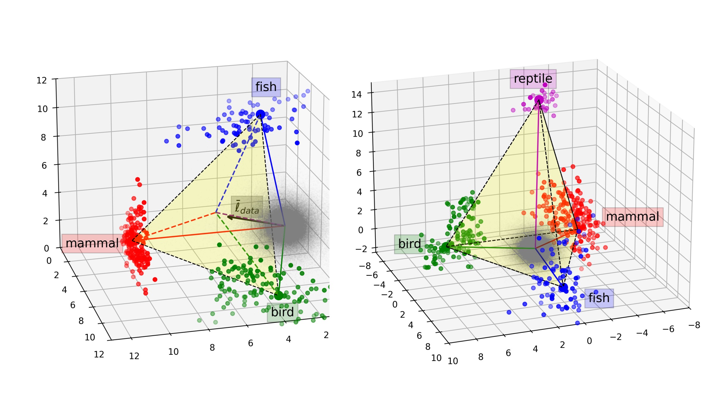
And this is what we get for completely random concepts:
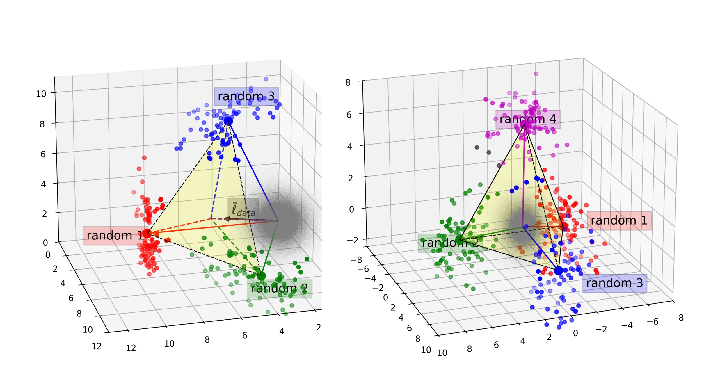
Thus, while categorical concepts form simplices, so do completely random, non-sensical concepts. Again, as we will show theoretically, randomly made categories are likely to form simplices and polytopes as well, because it is very easy to escape finite convex hulls in high-dimensional spaces.
Random Unembeddings Exhibit Similar Geometry
Here, we show that under the whitening transformation, even random (completely untrained) unembeddings exhibit similar geometry as the trained ones. This gives more empirical evidence that the orthogonality and polytope findings are trivially true and do not “emerge” during the training of a language model.
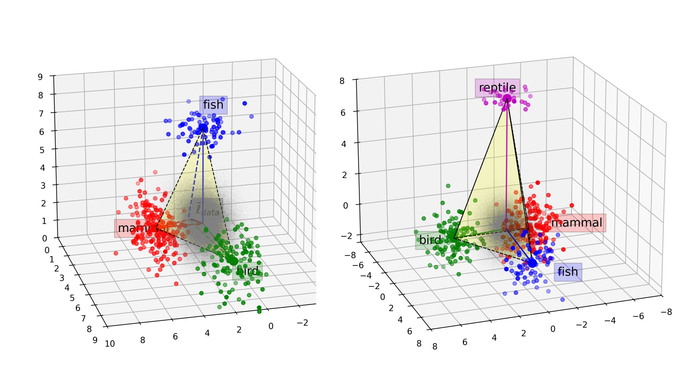
In the next section, we will theoretically show why these orthogonality and polytope results are trivially true in high-dimensions. Since the dimension of the residual stream of the Gemma model they used is $2048$, we claim many of their empirical findings are expected by default and do not show anything specific about the geometry of feature embeddings in trained language models.
Orthogonality and Polytopes Proofs in High Dimensions
Orthogonality and the Whitening Transformation
Many of the paper’s claims and empirical findings are about the orthogonality of various linear probes for concepts in unembedding space. Importantly though, “orthogonal” here is defined using an inner product after a whitening transformation. Under this definition, most concept probes are going to end up being almost orthogonal by default.
To explain why this happens, we will first discuss a simplified case where we assume that we are studying the representations in a language model with residual stream width $n$ equal to or greater than the number of tokens in its dictionary $k$. In this case, all the orthogonality results shown in Theorem 8 of the paper would exactly hold for any arbitrary concept hierachies we make up. So observing that the relationships in Theorem 8 hold for a set of linear concept probes would not tell us anything about whether the model uses these concepts or not.
Then, we will discuss real models like Gemma-2B that have a residual stream width smaller than the number of tokens in their dictionary. For such models, the results in Theorem 8 would not automatically hold for any set of concepts we make up. But in high dimensions, the theorem would still be expected to hold approximately, with most concept vectors ending up almost orthogonal. Most of the emprirical results for orthogonality the paper shows (see our section on empirical results) are consistent with this amount of almost-orthogonality that would be expected by default.
Case $n\geq k:$
The whitening transformation will essentially attempt to make all the vocabulary vectors as orthogonal to each other as possible. When the dimensionality $n$ is greater than the number of vectors $k$ (i.e., $n > k$), the whitening transformation can make the vectors exactly orthogonal.
Let \(\{ \mathbf{x}_1, \mathbf{x}_2, \dots, \mathbf{x}_k \} \in \mathbb{R}^n\) be zero-mean random vectors with covariance matrix $\Sigma$, where $n > k$. Then there exists a whitening transformation $W = \Sigma^{-1/2}$ such that the transformed vectors \(\{ \mathbf{y}_i = W\mathbf{x}_i \}_{i=1}^k\) satisfy:
\[\mathbb{E}[\mathbf{y}_i^\top\mathbf{y}_j] = \delta_{ij}\]where $\delta_{ij}$ is the Kronecker delta.
Proof:
$1.$ Consider the eigendecomposition $\Sigma = U\Lambda U^\top$, where \(\Lambda = \text{diag}(\lambda_1, \dots, \lambda_k)\) .
$2.$ Define $W = \Lambda^{-1/2}U^\top$. Then for any $i, j$:
\[\begin{aligned} \mathbb{E}[\mathbf{y}_i^\top\mathbf{y}_j] &= \mathbb{E}[(W\mathbf{x}_i)^\top(W\mathbf{x}_j)] \\ &= W\mathbb{E}[\mathbf{x}_i\mathbf{x}_j^\top]W^\top \\ &= W\Sigma W^\top = I_k \end{aligned}\]$3.$ If $n > k$, we can extend $W$ to an $n \times n$ orthogonal matrix that preserves the orthogonality property.
This matters, because if the dictionary embeddings are orthogonal, the relationships for concept vectors the paper derives will hold for completely made-up concept hierachies. They don’t have to be related to the structure of the language or the geometry of the original, untransformed unembedding matrix of the model at all.
As an example, consider a dictionary with $k=6$ tokens and a residual stream of width $n=6$. The tokens could, for instance, just be the first six letters of the alphabet, namely $\text{{a, b, c, d, e, f}}$. Following the convention of the paper, we will call the unembedding vectors of the tokens \(\ell_a, \ell_b,\dots, \ell_f\) .
Due the the whitening transformation, these vectors will be orthogonal under the causal inner product:
$\ell_a \cdot \ell_b=0$
$\cdots$
$\ell_e \cdot \ell_f=0$
The relationships described in Theorem 8 of the paper will then hold for any hierarchical categorization schemes of concepts defined over these tokens. The concepts do not need to be meaningful in any way, and they do not need to have anything to do with the statistical relationship between the six tokens in the training data.
For example, let us declare the binary concept \(\text{\{blegg, rube\}}\). Tokens $\text$ are “bleggs”, and tokens $\text$ are “rubes”. We further categorize each “blegg” as being one of $\text$, making a categorical concept. Token “a” is a “lant”, “b” is a “nant” and “c” is a “blip”.
We can create a linear probe $l_{\text{blegg}}$ that checks whether the current token vector is a ‘blegg’. It returns a nonzero value b_blegg/b_rube if the token is a ‘blegg’, and a value of 0 if it is a ‘rube’ (see Theorem 4 in the paper).
We could train the probe with LDA like the paper does, but in this case, the setup is simple enough that the answer can be found immediately. In the whitened coordinate system, we write:
$\ell_{\text{blegg}}=\ell_a+\ell_b+\ell_c$
$\ell_{\text{rube}}=\ell_d+\ell_e+\ell_f$
Constructing linear probes for ‘lant’ ‘nant’ and ‘blip’ is also straigthforward:
$\ell_{\text{lant}}=\ell_a$
$\ell_{\text{nant}}=\ell_b$
$\ell_{\text{blip}}=\ell_c$
Following the paper’s definitions, {‘lant’,’nant’, ‘blip’} is subordinate to {‘blegg’,’rube’}. We see that Theorems 8 (a,b,c) in the paper that illustrated in their Figure 2 will hold for these vectors.
8 (a) $\ell_{\text{blegg}}\cdot(\ell_{\text{lant}}-\ell_{\text{blegg}})=0$
8 (b) $\ell_{\text{blegg}}\cdot(\ell_{\text{lant}}-\ell_{\text{nant}})=0$
8 (c) $(\ell_{\text{blegg}}-\ell_{\text{rube}})\cdot(\ell_{\text{lant}}-\ell_{\text{nant}})=0$
So, in a $n$-dimensional space containing unembedding vectors for $n=k$ dictionary elements, Theorem 8 will hold for any self consistent categorisation scheme. Theorem 8 will also keep holding if we replace the unembedding matrix $W_{\text{unembed}}\in \mathbb{R}^{k\times n}$ with a randomly chosen full rank matrix. Due to the whitening applied by the ‘causal inner product’, the concepts we make up do not need to have any relationship to the geometry of the unembedding vectors in the model.
Case $n<k:$
If the model’s residual stream is smaller than the number of tokens in its dictionary, as is the case in Gemma-2B and most other models, the whitening transformation cannot make all $k$ unembedding vectors $x_1,\dots,x_k$ exactly orthogonal. So Theorem 8 will no longer be satisfied by default for all concept hierarchies and all unembedding matrices we make up.
However, if $n,k$ are large, the whitening transformation might often still be able to make most unembedding vectors almost orthogonal, because random vectors in high dimensional spaces tend to be almost orthogonal by default.
To see why this is the case, consider $k$ random vectors $\mathbf{x}_i \in \mathbb{R}^n$ for $i = 1, 2, \dots, k$ drawn from the unit sphere. We will show that as the dimensionality $n$ increases, these vectors become approximately orthogonal.
The expected value of the inner product $\langle \mathbf{x}_i, \mathbf{x}_j \rangle$ is:
\[\mathbb{E}[\langle \mathbf{x}_i, \mathbf{x}_j \rangle] = \mathbb{E}\left[\sum_{l=1}^n x_{il} x_{jl}\right] = \sum_{l=1}^n \mathbb{E}[x_{il} x_{jl}]\]The elements of the vectors have zero mean, so we have $\mathbb{E}[x_{il} x_{jl}] = 0$ for $i \neq j$. Therefore, the expectation value of the inner product is $\mathbb{E}[\langle \mathbf{x}_i, \mathbf{x}_j \rangle]$ is $0$.
The variance of the inner product is:
\[\text{Var}[\langle \mathbf{x}_i, \mathbf{x}_j \rangle] = \text{Var}\left[\sum_{l=1}^n x_{il} x_{jl}\right] = \sum_{l=1}^n \text{Var}[x_{il} x_{jl}] = \frac{1}{n}\]Thus, in high dimensions, the cosine of the angle $\theta$ between two random vectors has mean $0$ and deviation $\frac{1}{\sqrt(n)} \to 0$, meaning vectors will be nearly orthogonal with high probability.
In fact, the Johnson–Lindenstrauss lemma states that the number of almost orthogonal vectors that can be fit in $n$ dimensions is exponential in $n$.
So, going back to our example in the previous section, if the vectors $\ell_{a}, \dots,\ell_{f}$ are approximately orthogonal instead of orthogonal, then, the linear probes for the concepts {‘blegg’,’rube’}, {‘lant’,’nant’, ‘blip’} we made up would still mostly satisfy Theorem 8, up to terms $\mathcal{O}(\frac{1}{\sqrt{n}})$:
8 (a) $\ell_{\text{blegg}}\cdot(\ell_{\text{lant}}-\ell_{\text{blegg}})=\mathcal{O}(\frac{1}{\sqrt{n}})$
8 (b) $\ell_{\text{blegg}}\cdot(\ell_{\text{lant}}-\ell_{\text{nant}})=\mathcal{O}(\frac{1}{\sqrt{n}})$
8 (c) $(\ell_{\text{blegg}}-\ell_{\text{rube}})\cdot(\ell_{\text{lant}}-\ell_{\text{nant}})=\mathcal{O}(\frac{1}{\sqrt{n}})$
So, orthogonality between linear probes for concepts might be expected by default, up to terms $\mathcal{O}(\frac{1}{\sqrt{n}})$ that will become very small for big models with large residual stream widths $n$. To exceed this baseline, the causal inner product between vector representations would need to be clearly smaller than $\mathcal{O}(\frac{1}{\sqrt{n}})$.
High-Dimensional Convex Hulls are easy to Escape!
As for the polytope results in their paper (Definition 7, Figure 3 ), a random vector is highly likely to be outside the convex hull of $k$ vectors in high dimensions, so we should expect concepts to “form a polytope” by default.
Let \(\{ \mathbf{x}_1, \mathbf{x}_2, \dots, \mathbf{x}_k \} \in \mathbb{R}^n\) be $k<n$ independent random vectors drawn from the unit sphere. The convex hull of \(\{ \mathbf{x}_1, \mathbf{x}_2, \dots, \mathbf{x}_k \}\) is the set of points \(\sum_{i=1}^k \alpha_i \mathbf{x}_i\), where \(\alpha_i \geq 0\) and $\sum_{i=1}^k \alpha_i = 1$.
Since this polytope is contained in a $k$-dimensional subspace inside the larger $n$-dimensional space, its volume is $k<n$ dimensional rather than $n$ dimensional. So it has a n-dimensional Lebesgue measure of zero. So the probability that another random vector $\mathbf{z}$ lies inside this polytope will be zero. In the real world, our vector coordinates are floating point numbers of finite precision rather than real numbers, so the probability of $\mathbf{z}$ lying inside the polytope will not be exactly zero, but it will still be very small. Thus, it is not surprising that the polytopes spanned by linear probes for $k$ concepts do not intersect with linear probes for other concepts.
Even if we were to look at $k>n$ categorical concepts, Theorem 1 (Bárány and Füredi (1998)) shows, as described in
Discussion
Conclusion
We provide theoretical and empirical justification that the orthogonality and polytope results observed by recent works are a trivial consequence of the whitening transformation and the high dimensionality of the representation spaces.
A transformation where opposite concepts seem orthogonal doesn’t seem good for studying models. It breaks our semantic model of associating directions with concepts and makes steering both ways impossible. Thus, more work needs to be done in order to study concept representations in language models.
Related Works
Recent research has found multiple ways to extract latents representing concepts/features in a model’s activation space. We highlight some of them:
Linear Contrast/Steering Vectors
If we have a contrast dataset $(x^+, x^-)$ for a feature or behavior, we can use the contrast activations to get a $direction$ in a given layer’s activation space that represents the concept. This can also be used to steer models toward or away from it, as is shown in Representation Engineering
One can also extract linear function vectors in the activation space by eliciting in-context learning
Sparse Autoencoders (SAEs) and Variants
SAEs have been found to be a very scalable method to extract linear representations for a lot of features by learning a sparse reconstruction of a model’s activations
Unsupervised Steering Vectors
This work
Non-linear Features
While several important concepts are found to have linear representation latents (possibly due to the highly linear structure of the model’s architecture), not all features in a language model are represented linearly, as shown here
Future Work
We hope that our work points out various challenges toward a unified framework to study model representations and promotes further interest in the community to work on the same. Some important future directions this leaves us with are:
- A framework on how to think about representations that unifies how they’re obtained (contrastive activations, PCA, SAE, etc.), how they’re used (by the model), and how they can be used to control (eg. via steering vectors).
- How to figure out how well a given object (a direction, a vector, or even a black-box function over model parameters) represents a given human-interpretable concept or feature.
- If orthogonality and simplices are too universal and not specific enough to study the geometry of categorical and hierarchical concepts, then what is a good lens or theory to do so?
Lastly, instead of the whitening transformation (which leads to identity covariance), one can attempt to use an inverse, i.e., a coloring transformation using a covariance matrix that is learned directly from the data.
Reproducibility
All our results are completely reproducible and do not change with random seeds. The complete dictionaries for the two ablations we run (emotions and nonsense) are available here, and the code and hyperparameters we use are exactly the same as those used by the original authors, all of which is available on their public repository.
To reproduce our results, replace the original dictionary in the paper (for animals) with one of the others. For the random unembedding experiment, replace the unembedding matrix $W_U$ with torch.randn_like(W_U) and follow the rest of their methodology.