Models trained with unnormalized density functions: A need for a course correction
Training a generative model with energy or unnormalized density functions is considered an important problem for physical systems such as molecules. This provides a path to train generative models to sample from the much desired Boltzmann distribution in situations of data scarcity. As of late, several generative frameworks have been proposed to target this problem. However, as we show in the following blog post, these methods have not been benchmarked sufficiently well against traditional Markov Chain Monte Carlo (MCMC) methods that are used to sample from energy functions. We take the example of two recent methods (iDEM and iEFM) and show that MCMC outperforms both methods in terms of number of energy evaluations and wall clock time on established baselines. With this, we suggest a “course correction” on the benchmarking of these models and comment on the utility and potential of generative models on these tasks.
Introduction
AI for structural biology has a big-data problem. Simply put, there is a lack of sufficiently large datasets to train and deploy models that can generalize across diverse molecular systems and capture the full complexity of biomolecular interactions. The structural data available in the Protein Data Bank (PDB)
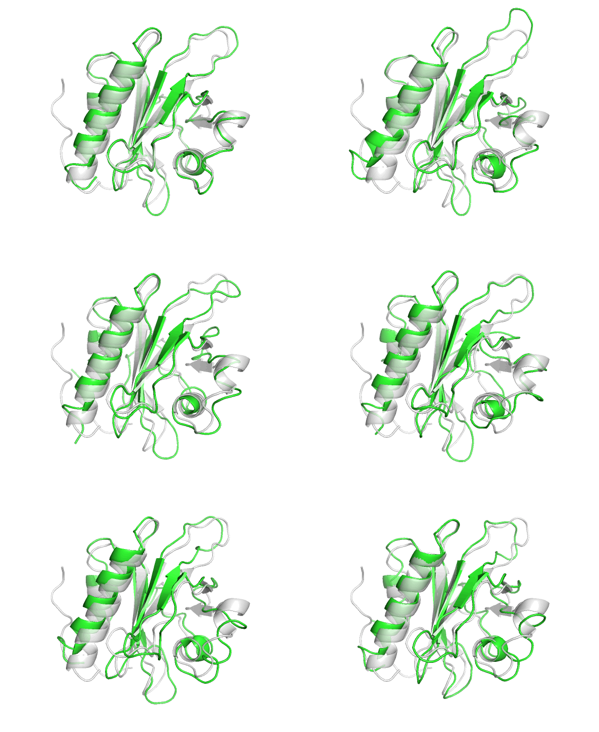
Molecular dynamics (MD) simulations can sample the conformational dynamics of molecular systems, but are constrained by sampling inefficiencies and the need for prohibitively long timescales. Addressing these limitations is essential to designing drugs that effectively modulate a protein’s function. Luckily, for physical systems such as molecules we have access to more information than just data to train generative models:
What if there was a thing called energy ? ;-)
— Adrian Roitberg 🏳️⚧️ (@adrian_roitberg) May 23, 2024
Yes that’s right, we know that for physical systems (molecules), the distribution of states (conformers) are characterized by their energy according the boltzmann distribution \(p(x) \propto exp(-\beta (\mathcal{E}(x)))\), where \(\mathcal{E}(x)\) is the energy of the state and \(\beta\) is a constant dependant on temperature. This motivates a paradigm of training generative models that can take advantage of the energy function.
Recently, a surge of deep learning generative models has aimed to address the challenges of sampling and data scarcity by adopting innovative, data-free approaches
A key consideration to take into account with generative models is to check if they outperform traditional methods for sampling from unnormalized density (energy) functions like Markov Chain Monte Carlo (MCMC). In this work, we compare iDEM and iEFM to MCMC on the same physical systems they were tested on and show that MCMC outperforms both methods while taking the same number of queries from the energy function. With this result, we suggest a “course correction” on the benchmarking of these models and propose different avenues where the development of these generative models would be useful.
Same Goals, Different Paths: Comparing iEFM and iDEM
iEFM and iDEM are quite similar in their implementation. While iEFM is an extension of flow matching
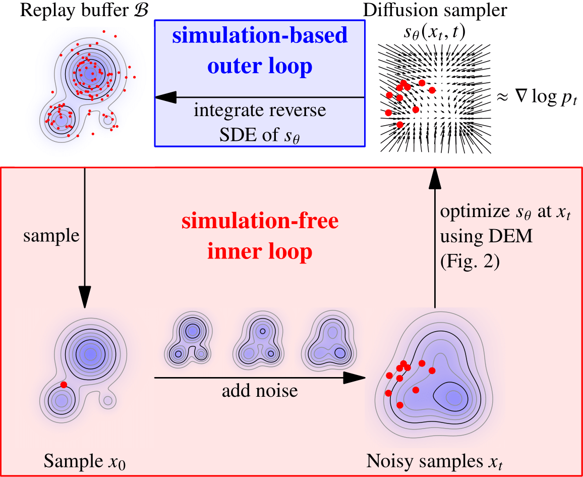
In an iterative process (Figure source: iDEM
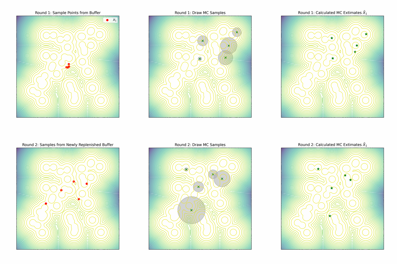
Developers of both methods, as well as others, have gravitated toward a standard set of toy systems for evaluation and benchmarking. While these systems are useful for early-stage development and illustrative purposes, we caution against over-reliance on them for robust benchmarking. As we will demonstrate, many related works employ MCMC samples of the equilibrium distribution but fail to use MCMC as a meaningful benchmark. In fact, MCMC often produces superior samples with faster runtimes on these systems compared to the proposed methods. Additionally, we show that the metrics commonly used for evaluation are poorly aligned with actual sample quality, further undermining their utility in assessing these methods.
MCMC and Sequential Monte Carlo
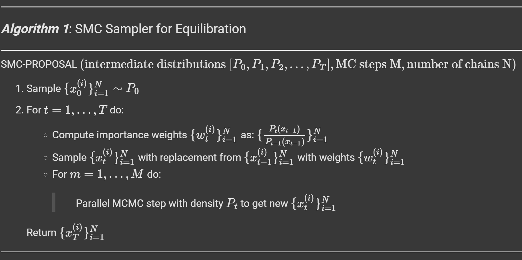
To generate samples for the test systems with MCMC, we follow a 2 step procedure. First we generate samples from a simple prior and try to quickly “equilibrate” them to the distribution of the desired density function through a short Sequential Monte Carlo (SMC) run, which is then followed on by regular MCMC for the remaining number of queries from the energy function.
MCMC steps are implemented as simple Metropolis Monte Carlo steps with a symmetric Gaussian proposal. The step sizes for the MCMC chains are decided by trying to maximize the value $\alpha*s$, where $\alpha$ is the acceptance rate and $s$ is the standard deviation of the gaussian proposal function.
SMC generates samples from a target density $p_T$ by creating a sequence of intermediate distributions that transition smoothly from the prior $p_0$ to $p_T$. At each step, samples are updated using a short MCMC chain ($M$ steps), reweighted to match the next intermediate density, and resampled to maintain particle diversity. The intermediates are typically constructed through linear interpolation between the unnormalized log-density functions (energy functions) of $p_0$ and $p_T$, enabling a gradual and efficient transformation of the samples toward the target distribution. The detailed algorithm for the same is shown in the algorithm block below.
Benchmark systems
Original work on iDEM was evaluated on a series of four increasingly complex benchmark systems. The simplest is a 2D Gaussian Mixture Model (GMM) comprising 40 equally-weighted Gaussians with identical covariance matrices and means uniformly distributed across a [-40, 40] box, serving as a basic test for mode coverage and sampling quality. The Double Well 4-particle system (DW-4) introduces greater complexity by modeling four particles in 2D space interacting through a pairwise double well energy function (figure below left). This system comes with symmetry properties, incorporating rotation, translation, and particle permutation invariance.
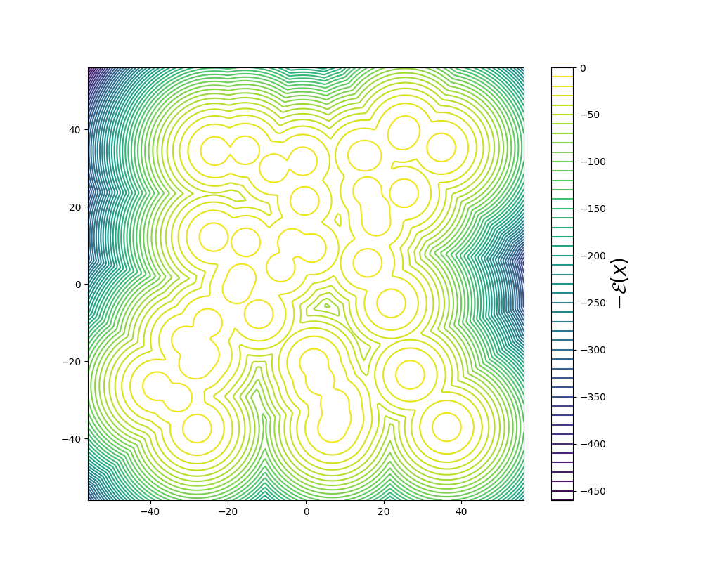
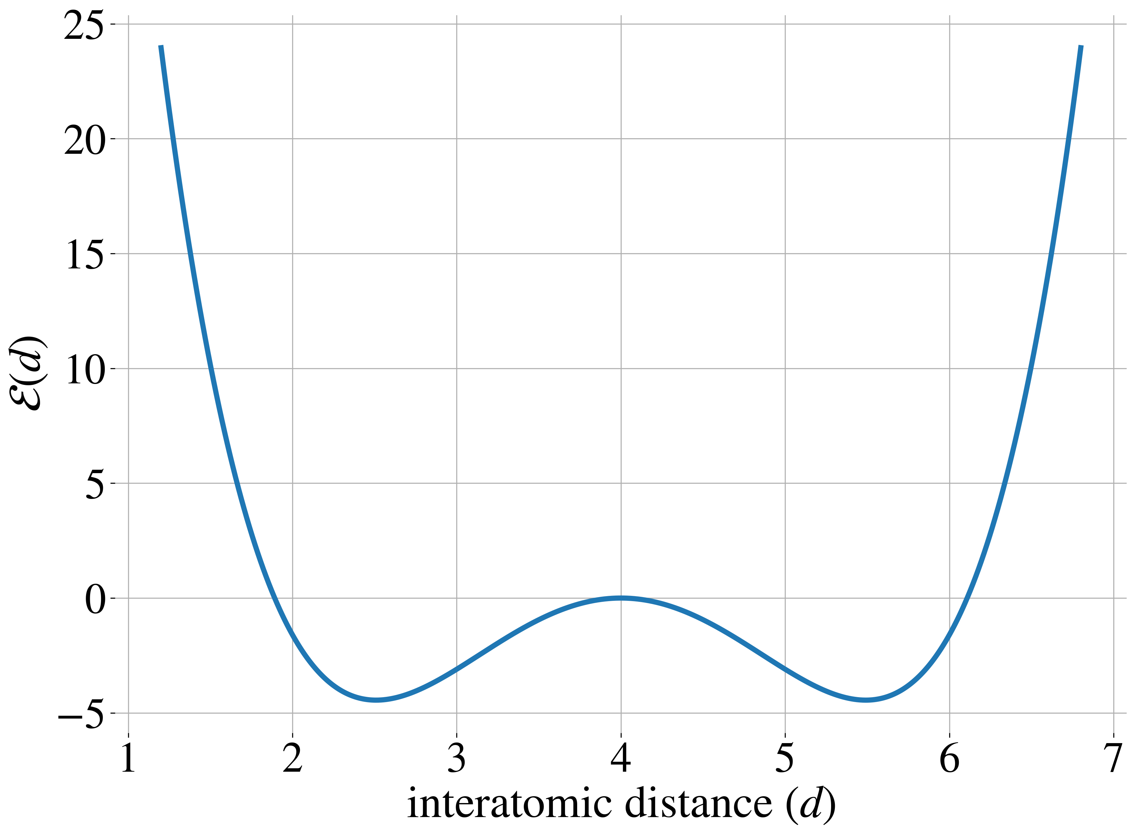
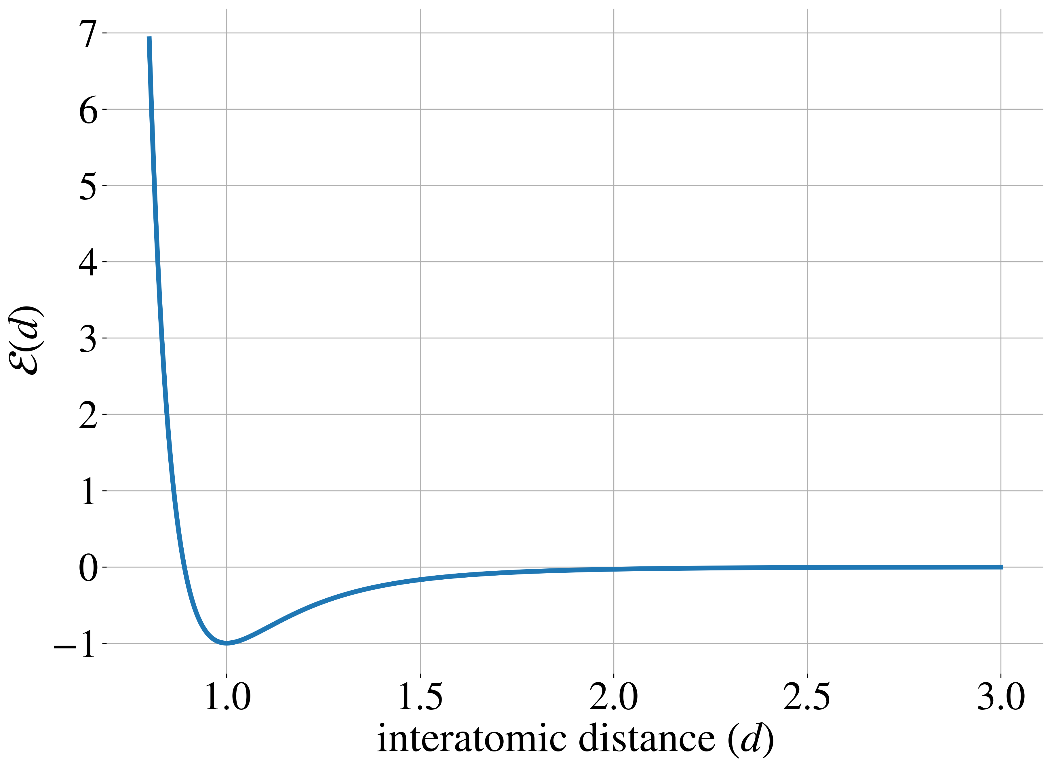
The most challenging benchmarks are two Lennard-Jones (LJ) systems that model interatomic interactions through a combination of attractive and repulsive potentials, supplemented by a harmonic oscillator term that tethers particles to their center of mass. The Lennard-Jones potential between two particles is shown in the figure above on the right. The LJ-13 system models 13 particles in 3D space (39 degrees of freedom), while the LJ-55 system handles 55 particles (165 degrees of freedom). These systems are particularly demanding due to their high dimensionality and the explosive nature of their energy function as interatomic distances approach zero.
Ground truth data for each system was generated using the following procedures:
- (GMM) The test set consists of 1000 samples generated directly from the known mixture distribution using TORCH.RANDOM.SEED(0). Since this is a well-defined mixture of Gaussians, true samples can be generated exactly without approximation.
- (DW4) The ground truth data comes from MCMC samples provided by Klein et al. (2023)
. The paper explicitly notes that while this might not be perfect ground truth, it’s considered reasonable for evaluation purposes. They specifically mention avoiding using an older dataset from Garcia Satorras et al. (2021) because it was biased, being generated from a single MCMC chain. - (LJ) Like DW-4, these systems use MCMC samples from Klein et al. (2023) as ground truth. The paper again notes they deliberately avoided using earlier datasets from Garcia Satorras et al. (2021) because these were biased, being generated from single MCMC chains.
A key point to note is that for the physical systems (DW-4, LJ-13, LJ-55), the ground truth data relies on MCMC sampling since exact sampling is intractable. Only the GMM system has true exact samples since its distribution is explicitly defined.
Experiment Details
iDEM was trained separately for all the 4 systems with 5 different seeds: GMM, DW4, LJ13, and LJ55. The iDEM models were trained using the default configs provided on their github repository: https://github.com/jarridrb/DEM. We only made one change so that our evaluations were consistent across the board. We ensured the evaluation batch size is equal to 1000 for all the systems.
iEFM was reimplemented to align as closely as possible with the algorithm described in the original manuscript. However, the absence of detailed experimental procedures and a publicly available codebase rendered a completely faithful reproduction unattainable. For instance, only the Optimal Transport (OT) variant of iEFM is evaluated here, as we were unable to successfully train Variance Exploding iEFM. OT-iEFM employs a different noise schedule for the conditional path probabilities compared to iDEM. Specifically, $P_t(x_t \mid x_1)$ uses a linear schedule $\sigma(t) = \sqrt{1 - (1 - \sigma_{\min})*t}$, while $q(x_1; x_t)$ employs $\frac{\sigma(t)}{t}$, where $\frac{1}{t}$ is clamped to avoid division by zero. For the variance clamping, a max value of 80.0 and 1.3 was used for the GMM and DW4 systems, respectively. By virtue of the optimal transport formulation, OT-iEFM produces straight path trajectories at test time, requiring significantly fewer integration steps than iDEM—30 steps compared to 1000. Apart from these differences, the following hyperparameters were left unchanged to ensure consistency with iDEM: num_estimator_mc_samples, num_samples_to_generate_per_epoch, eval_batch_size, optimizer/lr. We also note that the original authors of iEFM did not report any results on the Lennard-Jones systems. In our experiments, we found that OT-iEFM was unable to train successfully on these systems. The codebase of reimplimented iEFM is at https://github.com/countrsignal/idem_vs_iefm
To run MCMC chains, Klein et al. (2023b) identified the best value of the MCMC step size for the DW4 and LJ13 systems as 0.5 and 0.025. We found the best value for LJ55 to be 0.0075 and GMMs to be 1.25. Therefore, these are the step sizes we used to run MCMC chains on these four systems. To ensure that our MCMC chains had exactly the same number of energy evaluations as IDEM and IEFM, we ran batch_size*num_mc_estimates chains in parallel, where num_mc_estimates is the number of MC estimates the methods used per sample. We then ensured that the number of MC steps we took are equal to inner_loop_iterations*epochs, where inner_loop_iterations is the number of iterations of training the models went through before testing. This resulted in 512,000 parallel chains for GMM, DW4 and LJ13 and 12,800 parallel chains for LJ55. We ran 5 sets of such parallel chains for each system.
The initial samples for the chains on the DW4 and GMM systems were sampled from a uniform prior, and the initial samples for the LJ systems were sampled from an isotropic Gaussian; SMC involved creating 5 intermediate distributions for the DW4 and LJ13 and running the intermediate chains for 1000 steps each. LJ55 required 10 intermediate distributions with 2000 MC steps per distribution. GMMs required no intermediate distributions and no intermediate MCMC steps, just random sampling from a uniform prior and reweighting samples based on Boltzmann weights ($w(x) = \exp(-\mathcal{E}(x))$) did the trick.
Evaluation Method
We evaluate all the methods in two ways: we track the value of metrics as a function of queries from the energy function and time, and also report the metrics on samples generated at the end of training/MCMC runs. All the metrics are computed on batches of 1000 samples. For all our metrics we ensure that the number of queries from the energy function for the MCMC runs exactly match that used by IDEM/IEFM. To compute the results from the samples generated at the end of the runs, we take 5 batches of 1000 samples from 5 independent runs, resulting in mean and std values for the metrics obtained from 25 batches in total. To obtain the compute time of the runs, we take the time required for 1 iteration of training/MCMC sampling and multiply that by the total number of training/MCMC steps. All the experiments were done on NVIDIA L40 GPUs.
We evaluate all methods based on their ability to approximate the target distribution and key observables, such as energy and interatomic distance. Consistent with the approaches outlined in the iDEM and iEFM papers, we quantify the overlap between the model’s distribution and the target distribution using the Wasserstein-2 distance.
The Wasserstein-2 (W2) metric measures the distance between two probability distributions by quantifying the cost of optimally transporting one distribution to the other. Lower values of the W2 metric indicating closer alignment and higher values signaling greater divergence. It reflects both the positional differences and probability mass, making it a useful tool for assessing how well a model captures the target distribution.
It is calculated as the square root of the smallest possible average squared distance needed to transform one distribution into the other, while ensuring their overall structures remain consistent. Mathematically, the Wasserstein-2 (W2) metric measures the distance between two distributions $P$ and $Q$, with densities $p(x)$ and $q(x)$, as:
\[W_2(P, Q) = \left( \inf_{\pi \in \Pi(P, Q)} \int \|x - y\|^2 d\pi(x, y) \right)^{1/2},\]where $\Pi(P, Q)$ represents the set of all possible joint distributions (or “transport plans”) that have $P$ and $Q$ as their marginal distributions. A transport plan, $\pi(x, y)$, describes how the probability mass from $P$ is moved to match $Q$, while maintaining the overall structure of both distributions. In practice, the W2 metric is calculated by approximating the distributions as empirical histograms and solving a numerical optimization problem to find the transport plan that minimizes the total squared transportation cost.
For higher-dimensional systems, where the W2 metric becomes less intuitive to interpret, we focus on specific observables such as the energy and interatomic distance to provide more interpretable comparisons. The energy W2 distance computes how similar the distributions of energy of the test samples and generated samples are. This provides a notion of how well the sampler is able to capture the ensemble observations of the equilibrium distribution. Finally, the interatomic W2 distance is a projection of the position of samples along a 1 dimensional measure and therefore should match very well if the generated samples are close to the distribution of the test set.
Random sampling and reweighting is sufficient for GMMs
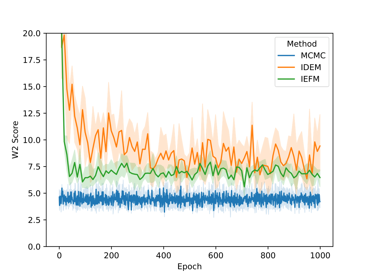
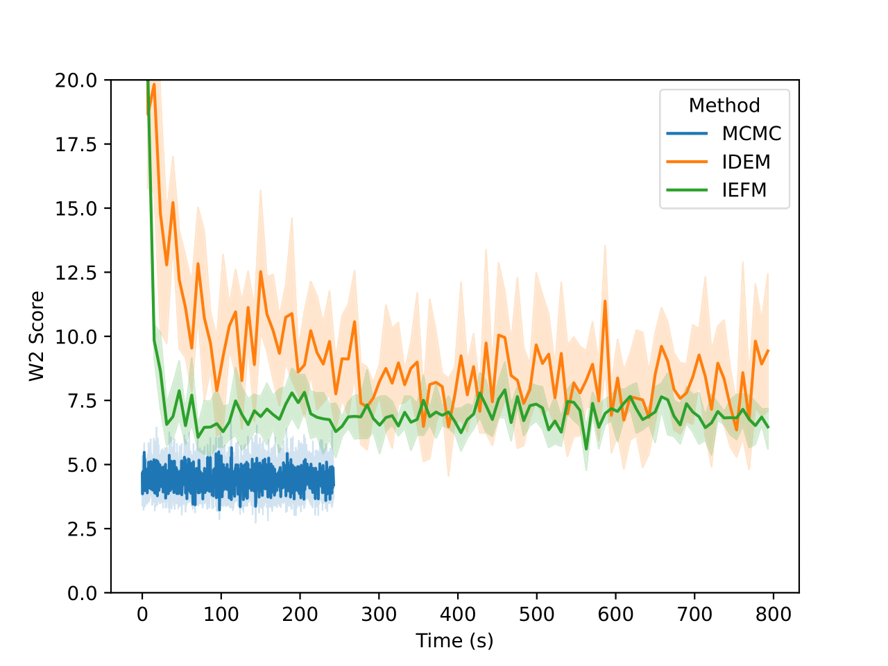
For the GMM system we initialize our MC chains using a uniform distribution with limits of [-45,45]. Since we are generating 512,000 samples on this 2D surface, we find that it’s sufficient to simply reweight the samples generated from the uniform prior according to their Boltzmann weights. We still continue to run MCMC chains after that for demonstration purposes. The figures above show that W2 scores of the runs as a function of number of training epochs and time. We define an “epoch” of a MCMC chain as the number of energy evaluations that are used to train an epoch of iDEM/iEFM.
| Method | W2 score |
|---|---|
| Ground truth | 4.159 ± 0.604 |
| IDEM | 7.698 ± 1.442 |
| IEFM | 7.364 ± 0.955 |
| MCMC | 4.219 ± 0.569 |
The table above contains the mean and std deviation of the W2 metrics vs the test set with 25 batches of 1000 samples obtained from different methods. Note that the W2 values for iEFM are higher than what is reported in the original paper. This discrepancy may arise from using a larger number of batches to evaluate the models, as well as potential imperfections in our implementation of iEFM. “Ground Truth” are samples generated directly from the GMM, thereby showing what the ideal values of the W2 score is. We see that only the MCMC method is able to get a W2 score similar to that of the ground truth. We also see that samples generated from the MCMC chains also more closely represent the ground truth in the figure below.
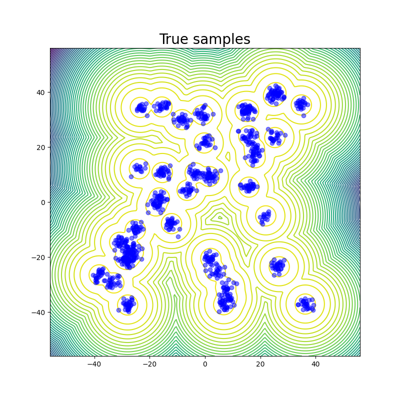
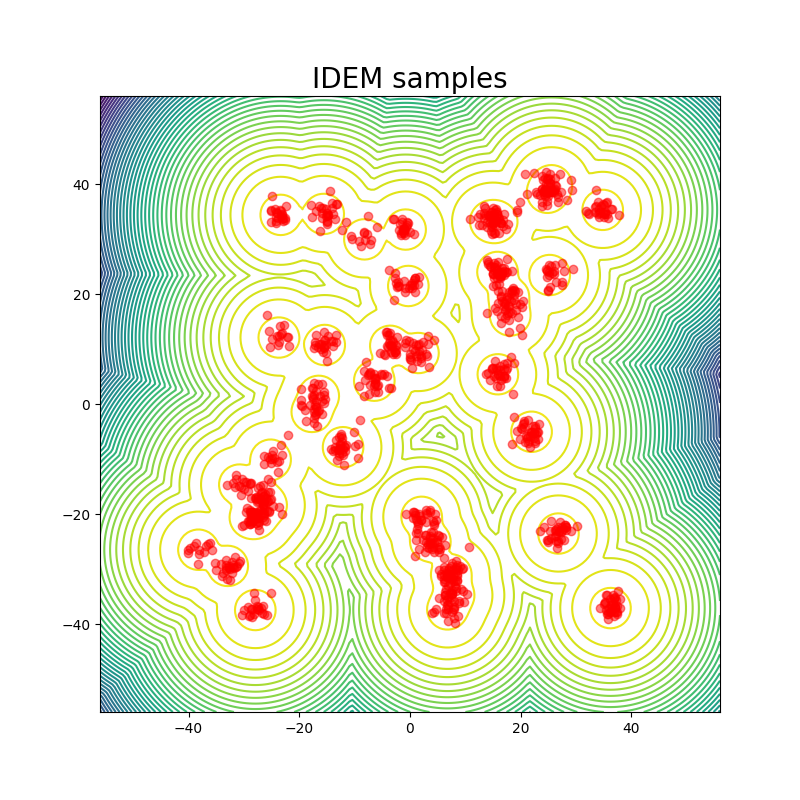
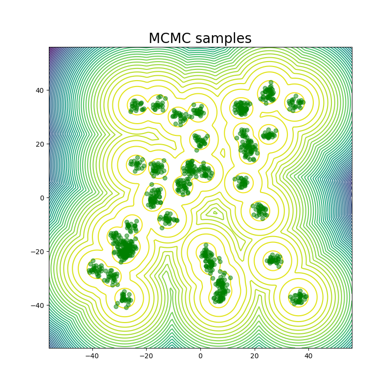
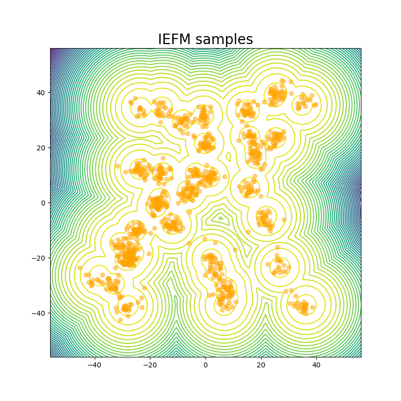
The fact that this system is just in 2 dimensions makes sampling from the distribution very easy; random sampling from a uniform prior and reweighting does the job, so it should not be considered a valid robust benchmark system for deep learning models for future works:
Everything works in 2D
— Frank Noe (@FrankNoeBerlin) August 30, 2024
Establishing new baselines for DW4, LJ13 and LJ55 with very long simulations
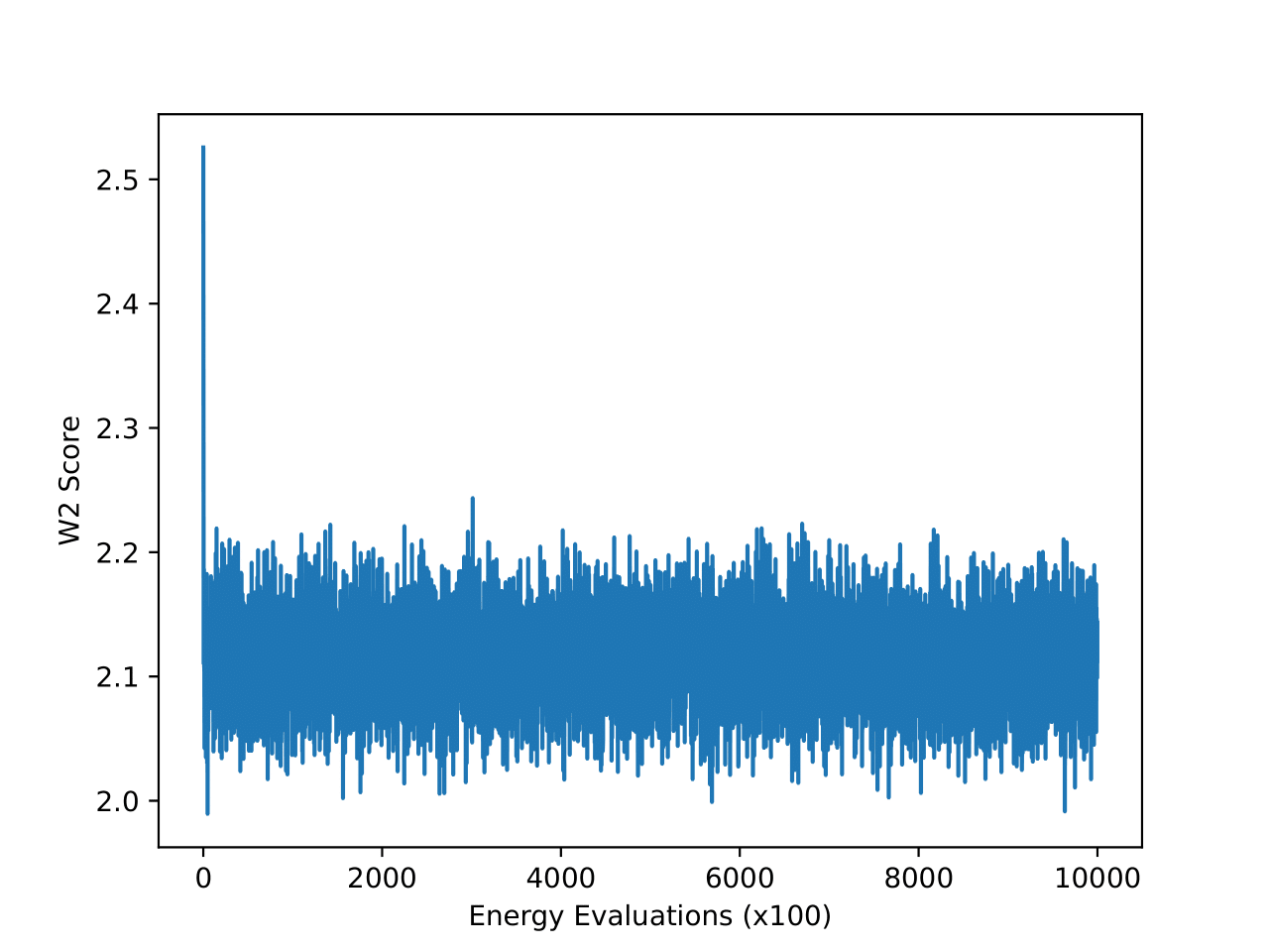
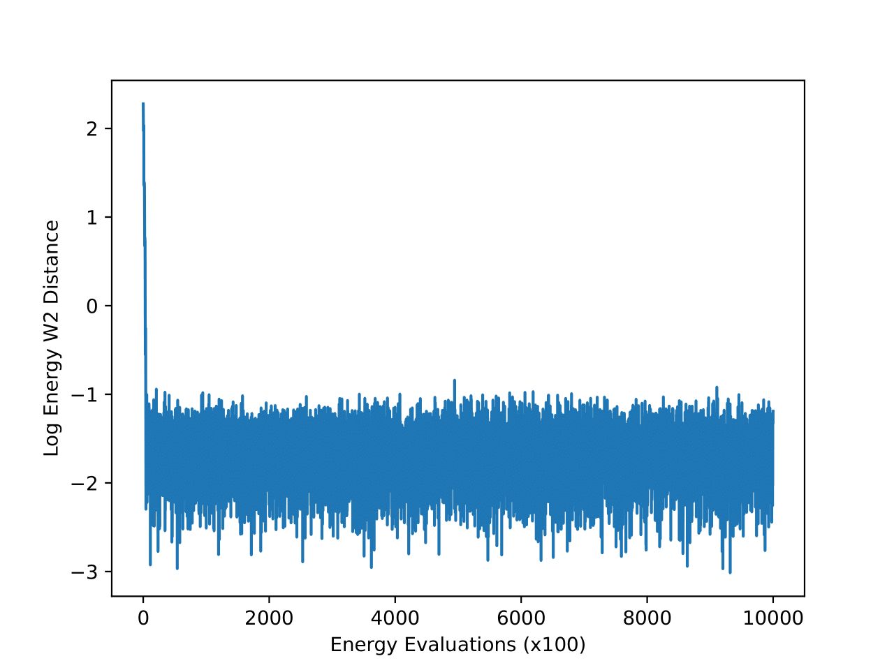
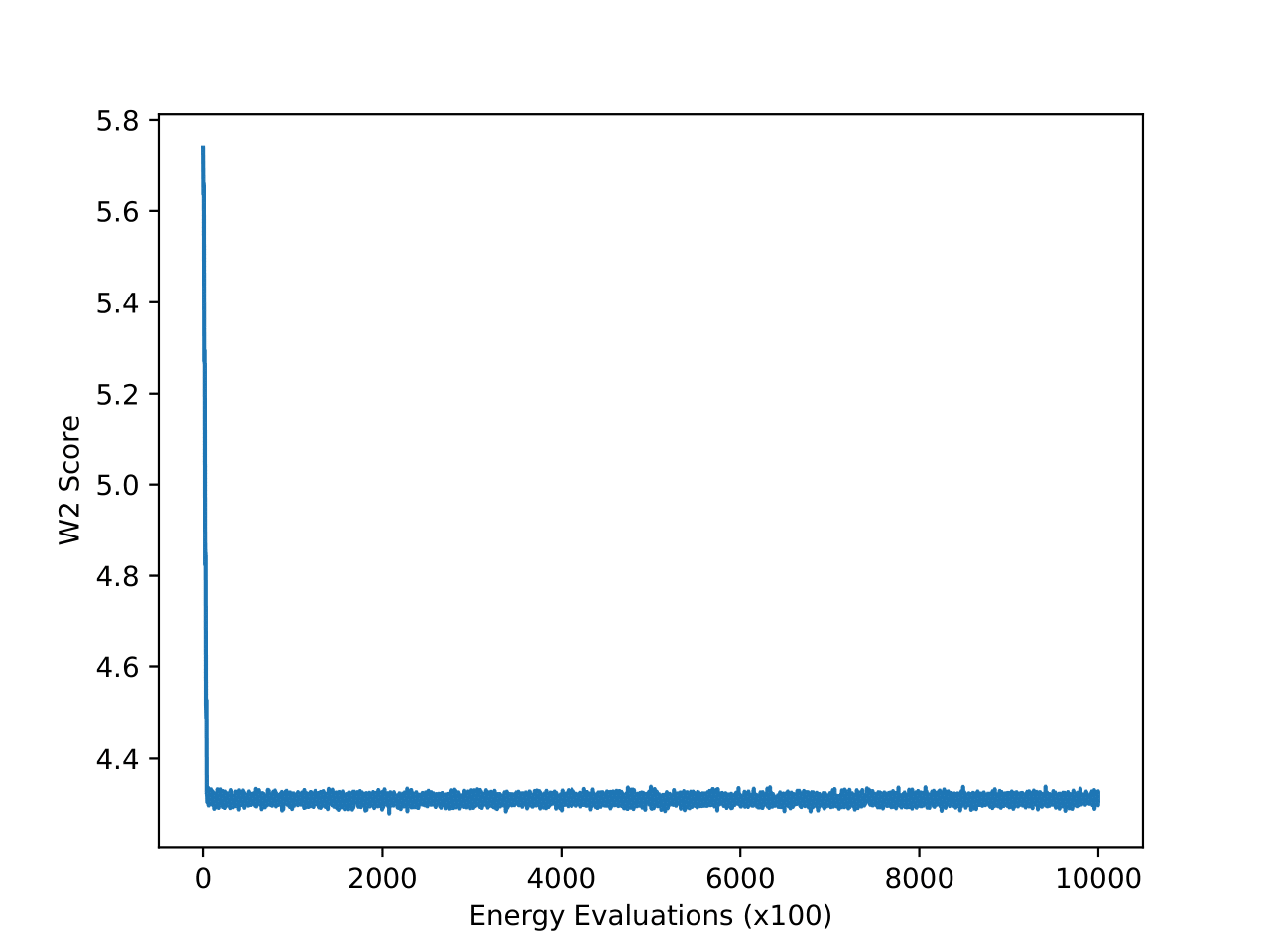
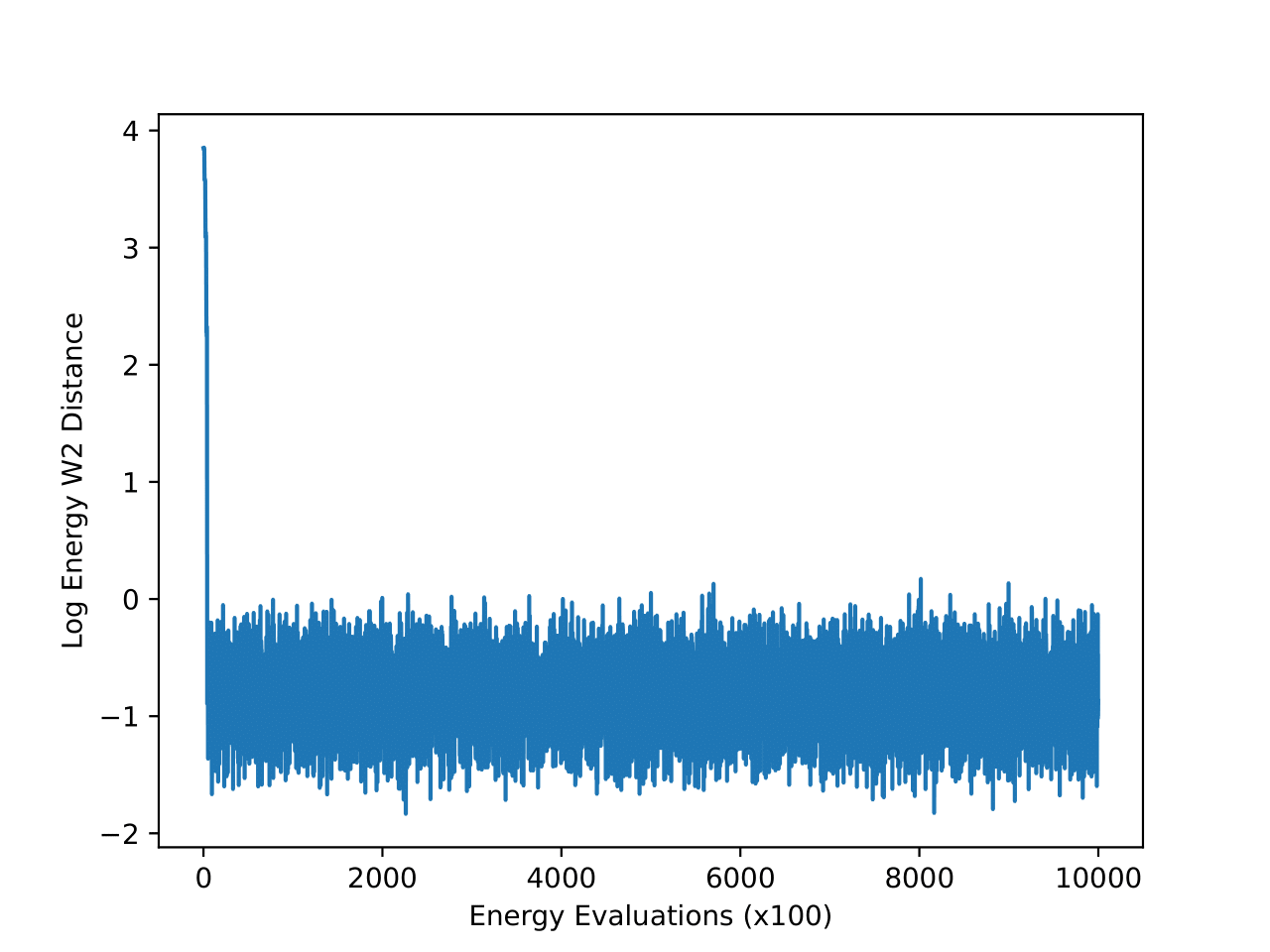
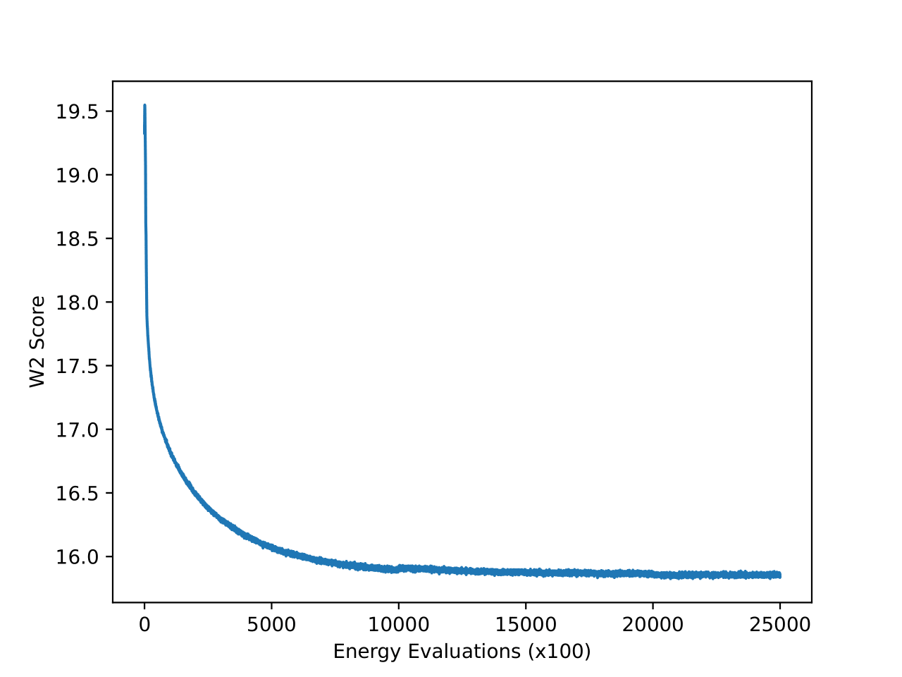
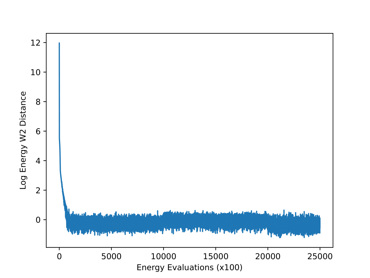
For the DW4, LJ13 and LJ55 systems we don’t have direct access to samples from the equilibrium distribution. Therefore, to create a strong “ground truth” baseline, we decided to run very long simulations on all of these systems and save the final state from all the simulations. For DW4 and LJ13, we ran 50,000 chains in parallel for a million steps, while for LJ55 we ran 12,800 chains for 2.5 million steps. This is much larger in contrast to the current test sets used by generative methods where the reference MC chain is run for about 200,000 steps. We assume that the combined end states of all these chains represent a distribution very close to the equilibrium distribution and can also be used as a new test set to benchmark on. In all the subsequent experiments, we compare the performance of all the methods on the set of end states of these long simulations (mentioned as “new reference” in the results tables).The W2 and energy W2 scores of the chains with respect to the reference test set (Klein et al.) used by iDEM and iEFM as a function of the number of MC steps are shown in the figures below. The convergence of all the runs on these metrics provides further evidence that the samples are close to the equilibrium distributions.
4-particle Double-Well Potential
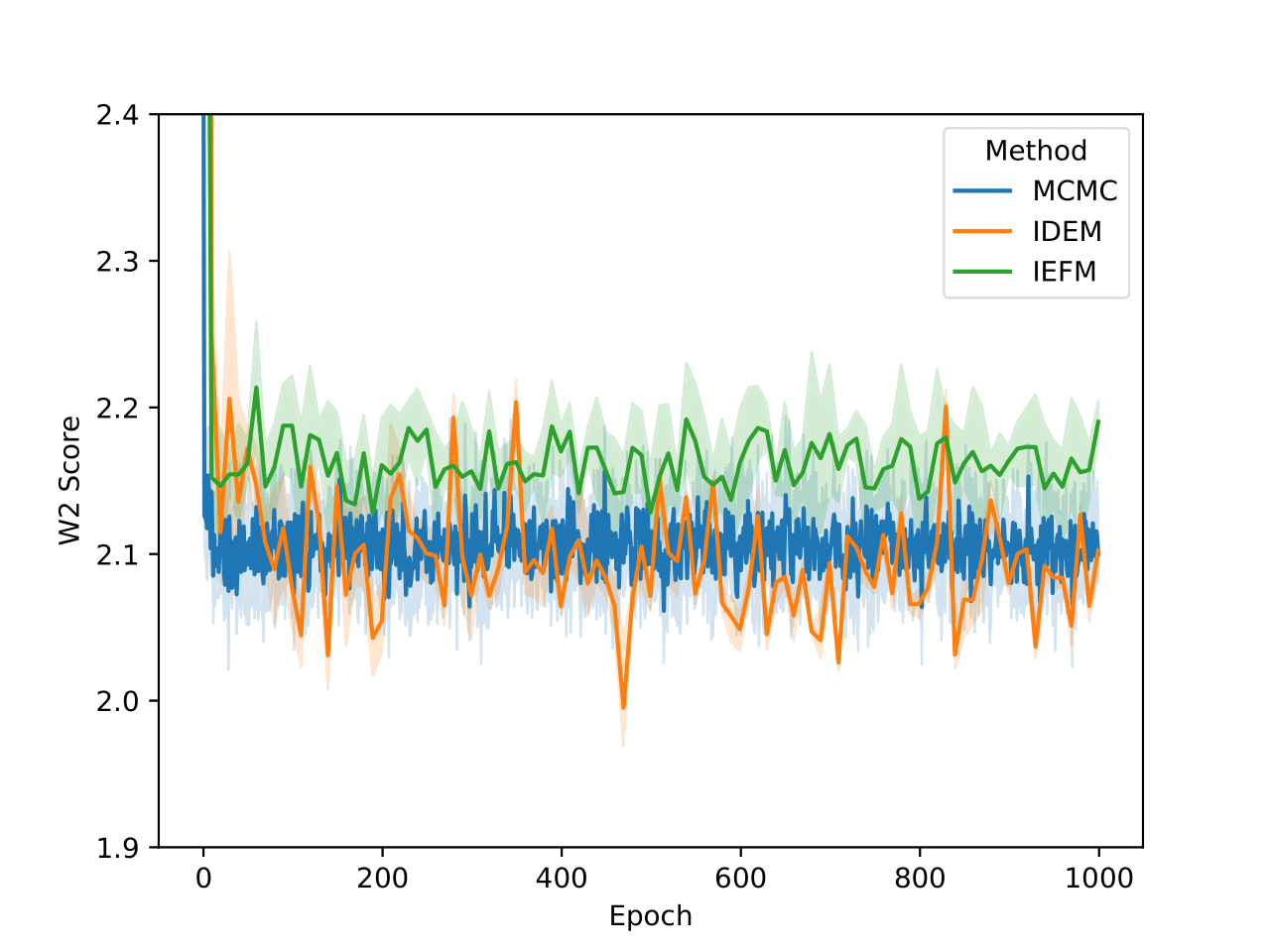
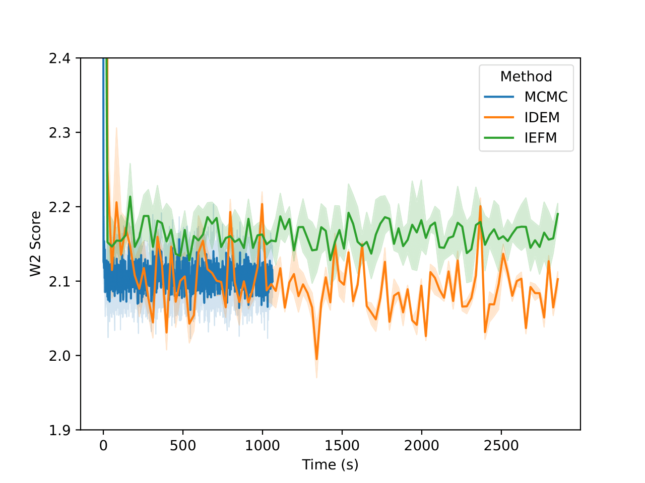
Examining the two plots (Figure 6), we observe W2 scores tracked over both epochs and wall-clock time. The MCMC method (blue line) stabilizes quickly around a W2 score of 2.1, exhibiting minimal variance, which reflects its robust and consistent sampling performance. In contrast, iDEM (orange line) displays more erratic behavior, with sharp dips and recoveries, though its average performance is similar to MCMC. Meanwhile, iEFM (green line) remains consistently above both methods with higher variance, indicating a lower and less reliable sampling quality. Notably, when plotted against wall-clock time, MCMC’s efficiency stands out, as it reaches and sustains optimal performance much faster than the neural methods.
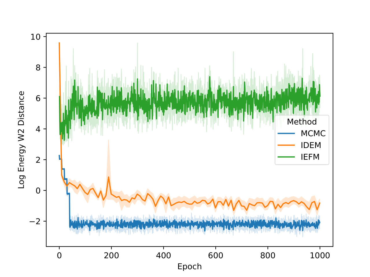
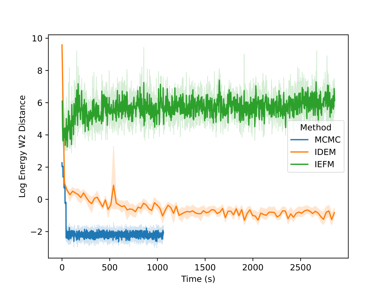
The energy W2 distance plots (Figure 7) further underscore the stark differences between the methods. MCMC rapidly converges to a low energy W2 distance and maintains this stability throughout. iDEM, however, takes significantly longer to converge and settles at a higher value of around 0, highlighting its less accurate energy sampling. iEFM performs the worst, with log energy W2 distances hovering near 6, demonstrating fundamental challenges in capturing the system’s energy landscape. The time-based comparison again highlights MCMC’s efficiency, achieving superior energy sampling far more quickly than its neural counterparts.
| Old Reference (Klein et al.) | New Reference (Long MCMC) | |||||
|---|---|---|---|---|---|---|
| Method | W2 | Energy W2 | Interatomic distance w2 | W2 | Energy W2 | Interatomic distance w2 |
| Long MCMC | 2.080 ± 0.030 | 0.157 ± 0.045 | 0.073 ± 0.012 | 1.883 ± 0.023 | 0.144 ± 0.044 | 0.017 ± 0.007 |
| IDEM | 2.054 ± 0.027 | 0.435 ± 0.153 | 0.139 ± 0.017 | 1.912 ± 0.021 | 0.590 ± 0.165 | 0.207 ± 0.014 |
| IEFM | 2.115 ± 0.035 | 3.852 ± 0.959 | 0.214 ± 0.014 | 1.928 ± 0.029 | 3.879 ± 0.909 | 0.145 ± 0.011 |
| MCMC | 2.068 ± 0.028 | 0.148 ± 0.048 | 0.067 ± 0.012 | 1.873 ± 0.032 | 0.132 ± 0.030 | 0.022 ± 0.012 |
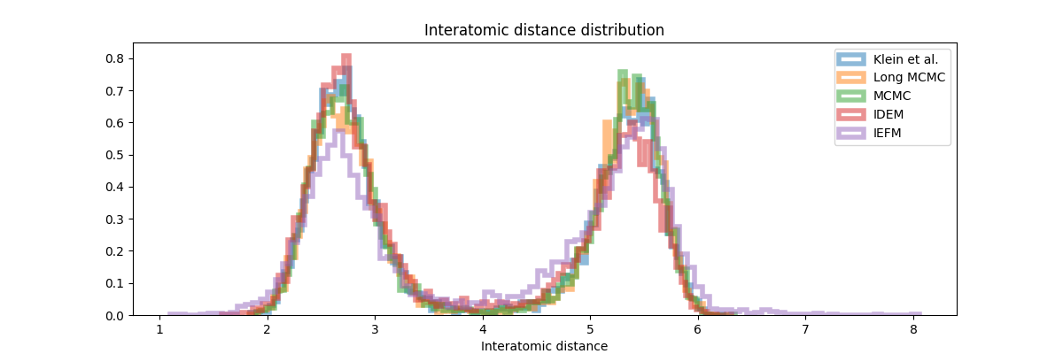
The quantitative results (Table 2) and distribution plots (Figure 8, 9) provide the most comprehensive insight into performance. Across all metrics, MCMC consistently achieves the best scores when compared to both old and new reference data. The distribution plots reveal key details: while iDEM captures the general shape of the interatomic distance distribution relatively well it still mismatches the peak height on the right. iEFM exhibits even more clear deviations in peak heights and locations. The energy distribution plot paints an even clearer picture—MCMC aligns closely with the reference distribution, whereas iDEM and iEFM show substantial discrepancies, particularly in the higher energy regions.
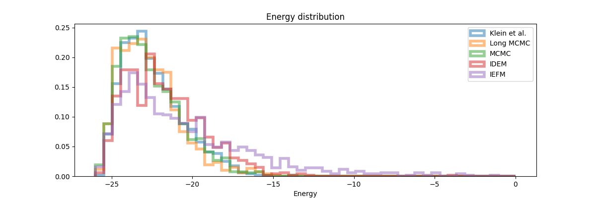
These findings suggest that while neural methods like iDEM and iEFM represent innovative steps forward in molecular sampling, they remain outperformed by the reliability and efficiency of well-tuned MCMC methods. The data strongly indicate that the added complexity of neural approaches does not yet translate into practical advantages over traditional methods, particularly for these benchmark systems.
13-Particle Lennard Jones System
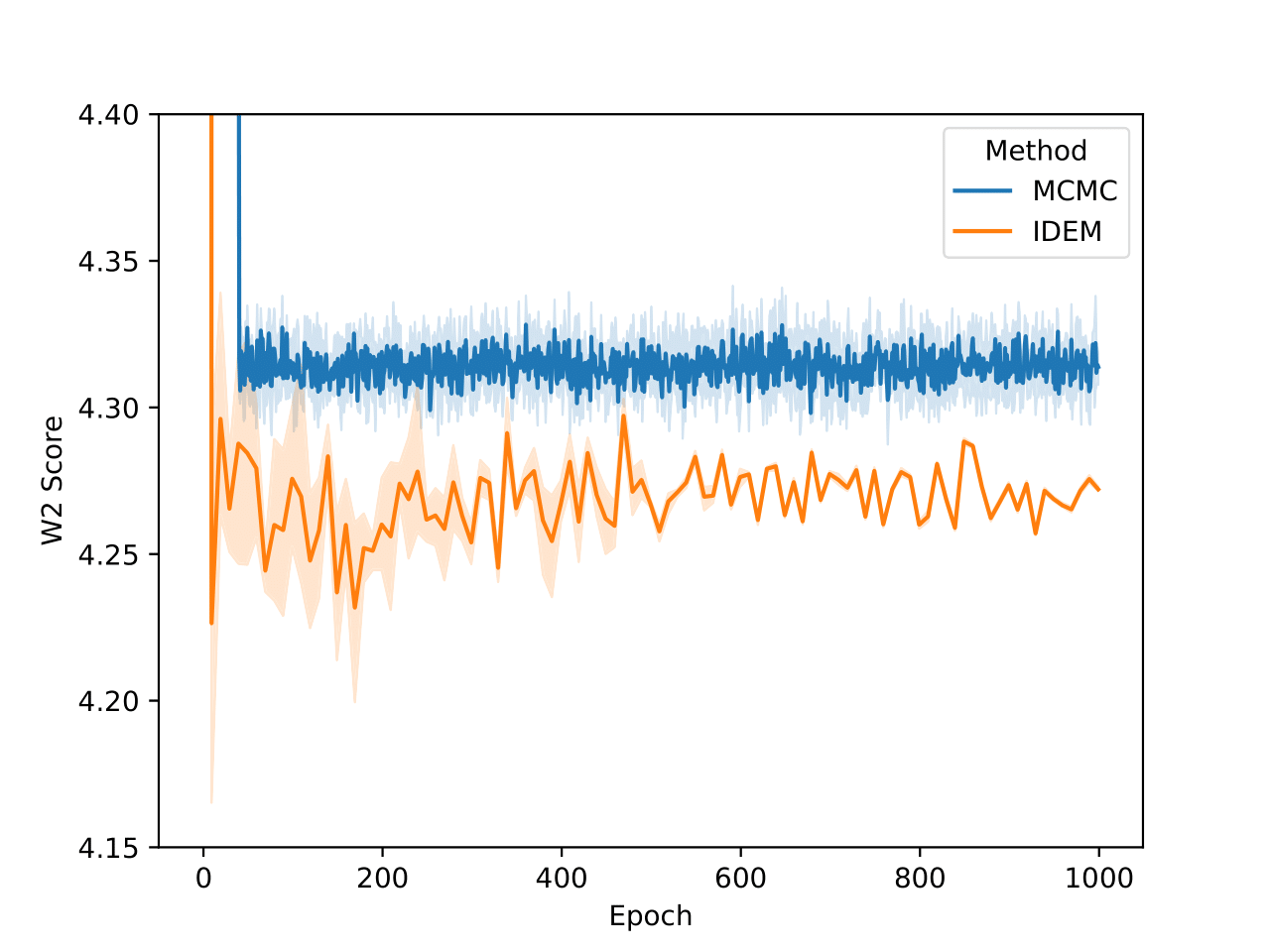
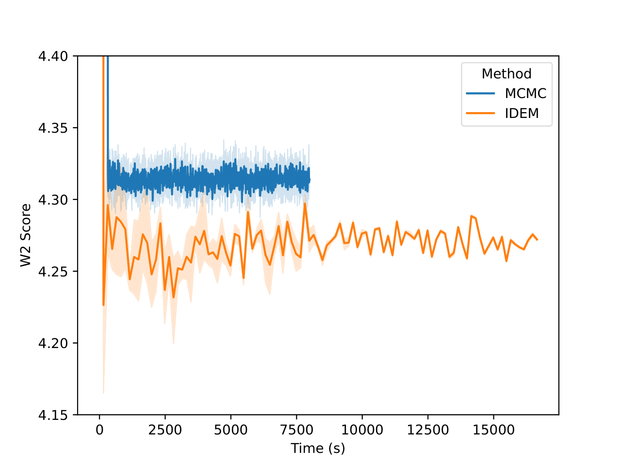
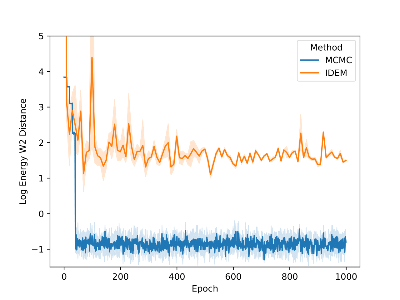
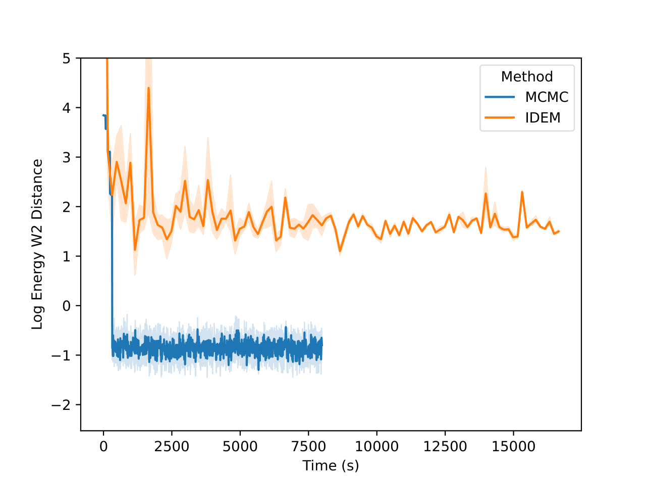
On the LJ13 system we observe that the MCMC runs actually get a higher W2 score than the IDEM runs (Figure 10). However, we posit that for higher dimensional systems, W2 between positions of data samples is not a good measure for the distance between two distributions. This is because even the long MCMC chains, having run for a million steps, do not attain a better W2 score than IDEM. In fact, from Figure 5, we can see that the W2 score for the long MC chain stabilizes and converges at a value of 4.31. Furthermore, the W2 score is only an upperbound on the best W2 score for a set of samples, as the current metric does not take rotations of the system and permutations of the particles into account. Moreover, both the short and the long MCMC chains have a much lower energy W2 value when compared to the reference test (Klein et al.) than iDEM, which indicates that they are better predictors of ensemble properties despite having a higher W2 score.
| Old Reference (Klein et al.) | New Reference (Long MCMC) | |||||
|---|---|---|---|---|---|---|
| Method | W2 | Energy W2 | Interatomic distance w2 | W2 | Energy W2 | Interatomic distance w2 |
| Long MCMC | 4.312 ± 0.007 | 0.457 ± 0.120 | 0.004 ± 0.002 | 4.298 ± 0.007 | 0.544 ± 0.167 | 0.005 ± 0.002 |
| IDEM | 4.266 ± 0.007 | 5.204 ± 1.788 | 0.024 ± 0.002 | 4.253 ± 0.005 | 4.73 ± 1.928 | 0.028 ± 0.003 |
| MCMC | 4.312 ± 0.005 | 0.516 ± 0.119 | 0.003 ± 0.001 | 4.297 ± 0.009 | 0.531 ± 0.171 | 0.006 ± 0.002 |
In Table 3, we also benchmark both the methods on the test set generated from the long MCMC chain that has been run for a million steps. Working under the assumption that the long MCMC chain is close to convergence, we can consider the metric values generated by it on both test sets as the best attainable values on this system. Therefore, we can consider the best methods to be the ones that have the closest metric values to that provided by the long MC chain. From the table, it is visible that the MCMC method does best in this regard. Furthermore, MCMC has much better energy and interatomic distance W2 scores than iDEM on both reference sets.
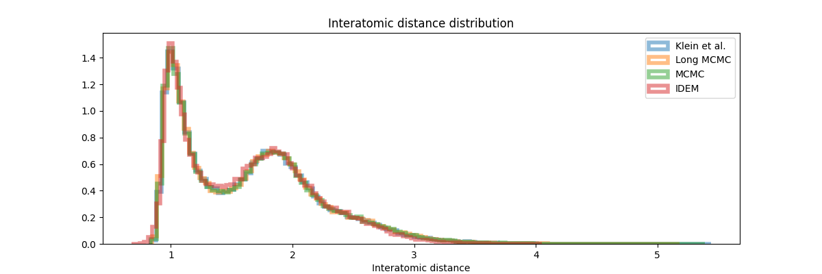
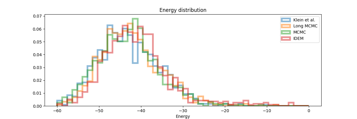
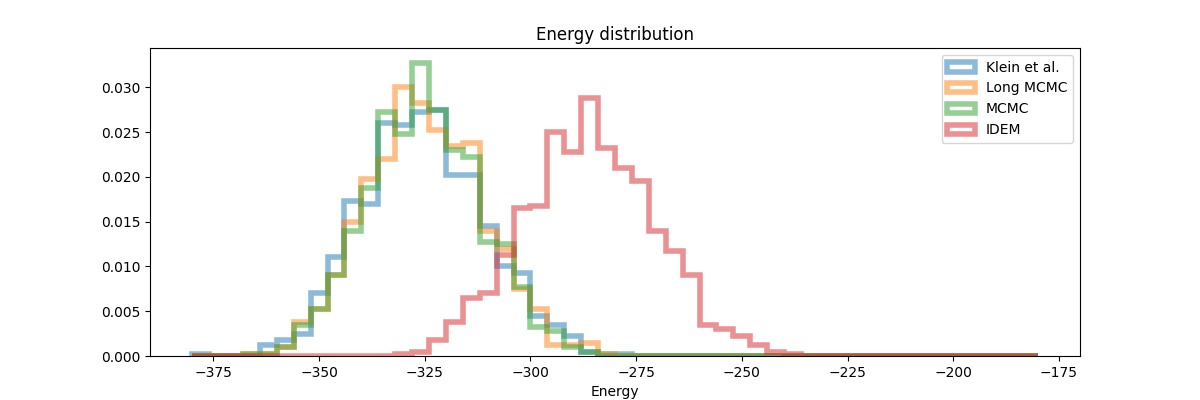
Finally, in the histogram plots, it’s clear that the IDEM energy plot is right shifted as compared to both the reference sets that have good agreement among themselves and with the shorter MCMC chains. iDEM also has less agreement on the interatomic distance histogram as compared to the other methods. Considering all the metrics and distributions, we conclude that MCMC outperforms iDEM on this system.
55-Particle Lennard Jones System
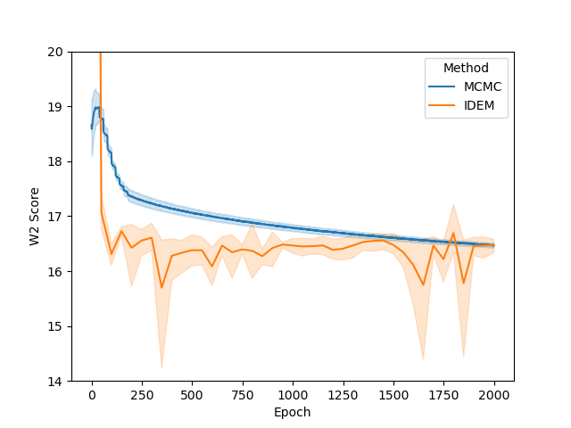
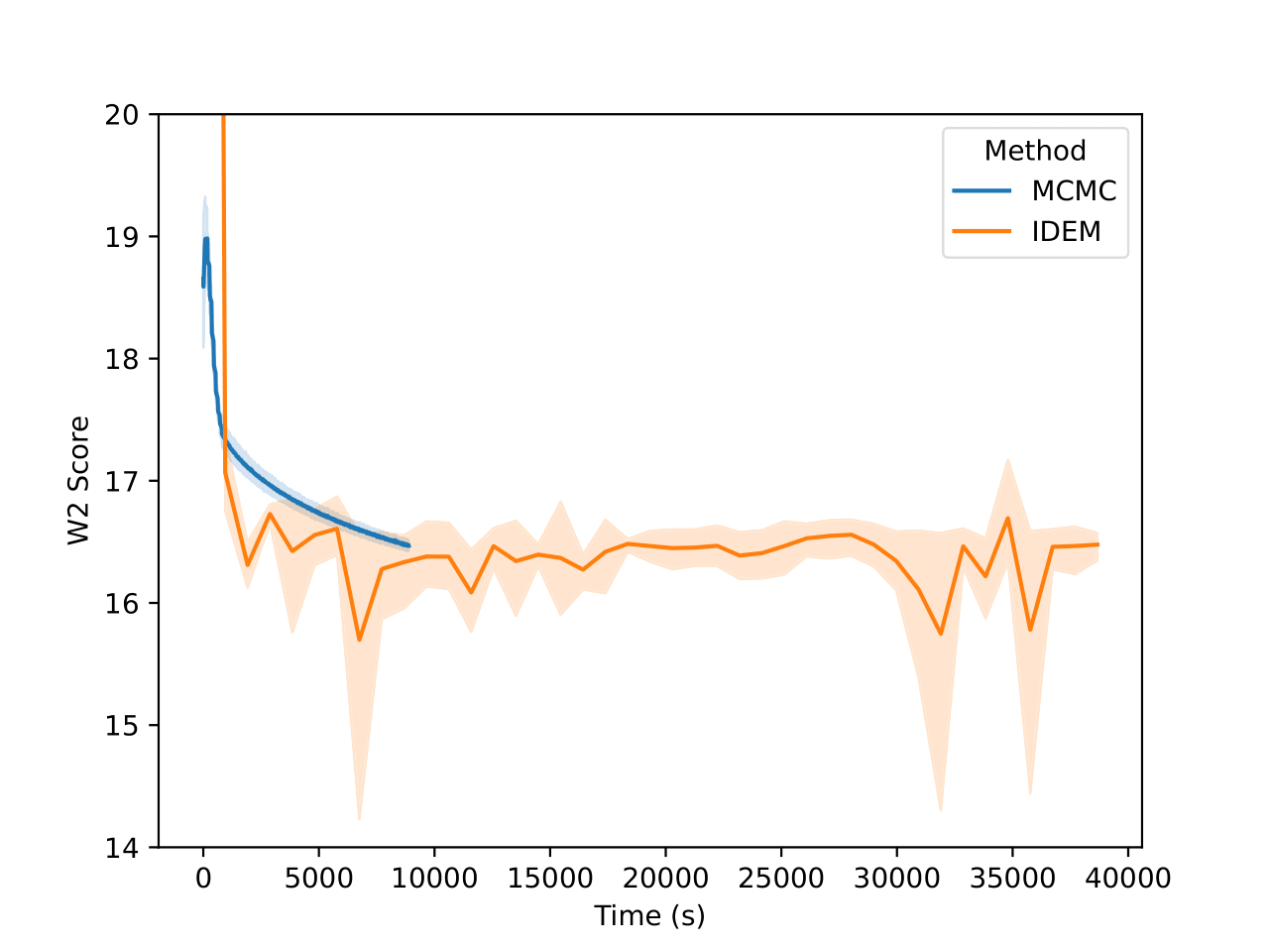
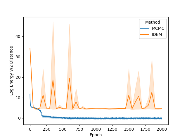
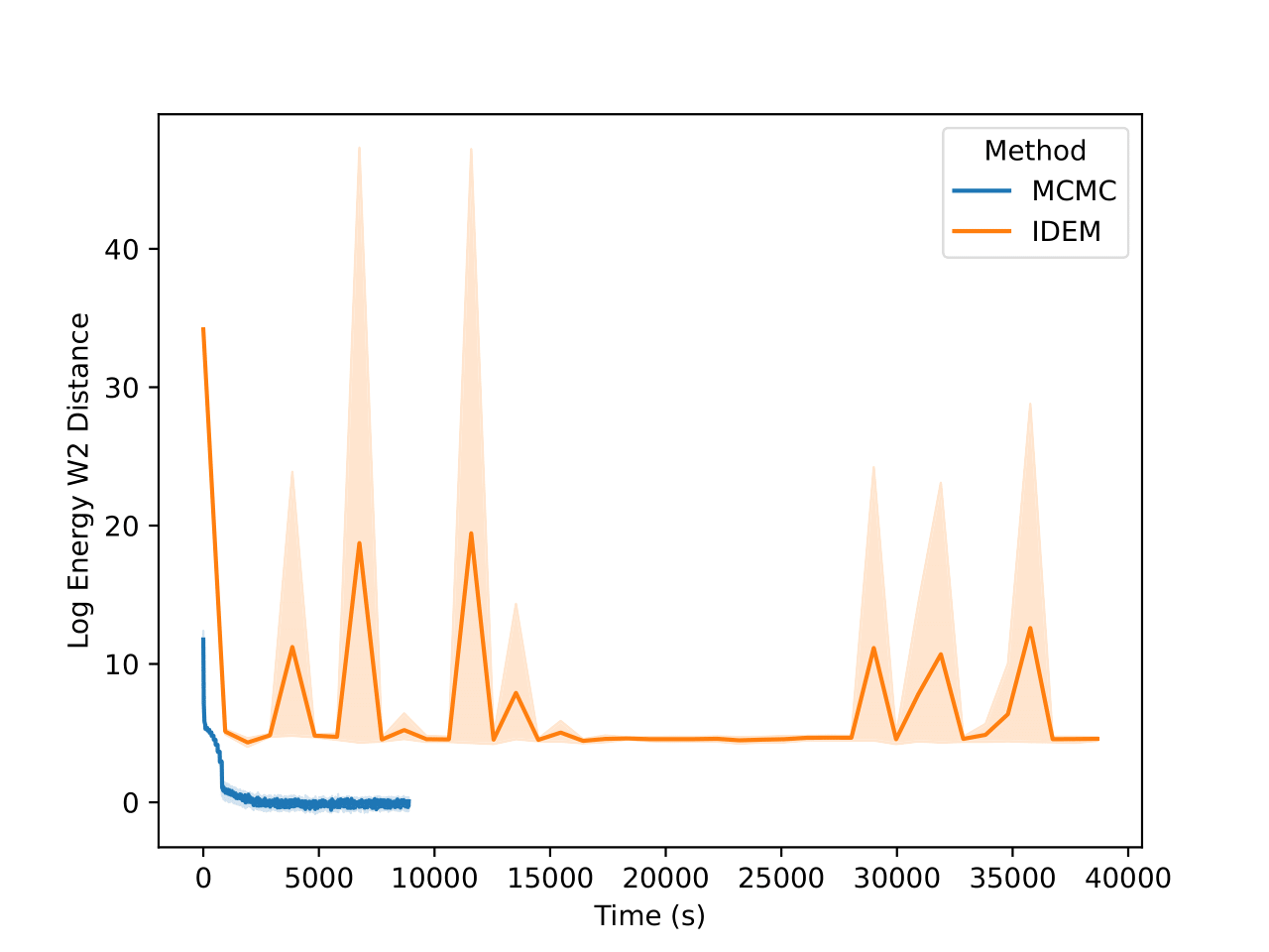
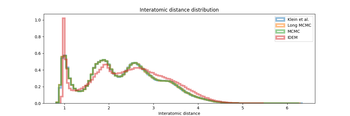
From the figures, we notice similar but exaggerated trends that we observed in the LJ13 systems. The MCMC chains return a higher W2 score but have a significantly lower energy W2 score. Therefore, we emphasize the importance of visualizing the distribution of observations (such as energy and interatomic distance) as the complexity of systems increases with increase in dimensions.
| Old Reference (Klein et al.) | New Reference (Long MCMC) | |||||
|---|---|---|---|---|---|---|
| Method | W2 | Energy W2 | Interatomic distance w2 | W2 | Energy W2 | Interatomic distance w2 |
| Long MCMC | 15.923 ± 0.009 | 0.931 ± 0.243 | 0.001 ± 0.0006 | 15.779 ± 0.007 | 0.680 ± 0.211 | 0.001 ± 0.0005 |
| iDEM | 16.143 ± 0.122 | 21.704 ± 15.174 | 0.085 ± 0.033 | 16.054 ± 0.125 | 21.531 ± 15.314 | 0.084 ± 0.034 |
| MCMC | 16.48 ± 0.0497 | 0.872 ± 0.237 | 0.001 ± 0.0005 | 16.42 ± 0.026 | 0.907 ± 0.391 | 0.002 ± 0.0009 |
From the table above and figures below, it is clearly visible that iDEM does not converge to generating the equilibrium distribution; we see huge deviations from what could be considered the ideal energy W2 and interatomic W2. The energy distribution particularly has much lower overlap to the references as compared to all the other methods. Furthermore, iDEM is not even able to obtain the overall correct shape of the interatomic distances despite having the same number of energy evaluations as MCMC.
Closing thoughts - the role that these models have to play
Our analysis offers a sobering assessment of the current state of neural network-based samplers for molecular systems. Despite the growing interest in methods like iDEM and iEFM, our results show that these approaches fail to outperform well-tuned MCMC methods in terms of both sampling quality and computational efficiency. This finding is particularly significant because, for neural samplers to justify their additional complexity and computational overhead, they must demonstrate clear and consistent advantages over traditional methods — a standard that these approaches have yet to meet. A possible solution to having more computationally efficient method would be to learn an approximate distribution specified by a complicated energy function and obtain the right distribution through a simple reweighting, as demonstrated by Klein et al.
However, this critique should not also be viewed as a wholesale rejection of such neural approaches in molecular sampling. Rather, it suggests a needed shift in research focus. One promising direction lies in leveraging neural networks’ capacity for transfer learning. While MCMC methods are often system-specific, and require long chains on every new system, neural networks could potentially learn generalizable sampling strategies that transfer across different molecular systems. This transferability could provide a compelling “inference time” advantage over traditional MCMC methods, even if the training cost is significantly higher than running a MCMC chain on a single system. This has already been demonstrated in works such as TimeWarp
A critical limitation of current neural approaches like iEFM and iDEM lies in their reliance on weighted averages of noisy samples. This becomes particularly problematic when dealing with real molecular systems, where energy landscapes can be extremely steep and sampling noise can lead to explosive gradients. Future work might address this by reconsidering how noise is incorporated into these models - for instance, by defining noise on a Riemannian manifold that respects the geometric constraints of molecular systems
Acknowledgements
This work is funded through R35GM140753 from the National Institute of General Medical Sciences. The content is solely the responsibility of the authors and does not necessarily represent the official views of the National Institute of General Medical Sciences or the National Institutes of Health.