Building Blocks of Differentially Private Training
In this blog, we introduce the building blocks of training a neural network in a differentially private way.
Introduction
Differential privacy (DP) is a powerful mathematical framework that allows us to reason about privacy in any process that takes input data and produces some output. Whether we’re computing simple statistics, training machine learning models, or generating synthetic data, DP provides quantifiable privacy guarantees by carefully introducing randomness into our computations.
In this post, we’ll focus on one instance of DP: training a neural network with differential privacy guarantees for the training data. Why should you care? Consider these scenarios:
- Medical records being used to train diagnostic systems
- Private messages helping improve language models
- Financial transactions training fraud detection algorithms
In each case, we have a process that takes sensitive individual datapoints as input and outputs model parameters, which could potentially reveal information about that training data. A deployment can bring huge social benefits if the model works well, but it could also lead to ugly privacy breaches if the training data can be inferred.
We’ll explore this challenge through a simple yet concrete example: training a two-layer neural network on a simple classification dataset with DP guarantees. While simple, we try to illustrate some of the challenges and solutions in DP deep learning. Specifically, we’ll consider DP guarantees over individual training examples - meaning an observer shouldn’t be able to tell whether any particular image-label pair was used during training, even with complete access to the model parameters.
Why this blog: The main motivation for this blog is to introduce DP in a concrete but simple setting. Even in this very simple setting, training a DP model requires a set of tricks. By introducing a subset of these tools, we aim to give the broader community a very limited, yet not completely out-of-touch, perspective on the progress and challenges of DP training. For a broader guide on DP and some best practices, we recommend the review
Some Foundations of Differential Privacy
In principle, DP is about plausible deniability. The key insight is this: an observer shouldn’t be able to determine whether any particular individual datapoint was used to train a model, even if they:
- Have complete access to the model’s parameters
- Know all other training datapoints
- Have unlimited computational power
This protection should also hold true regardless of what other information the observer might have. That’s a nice list of requirements, let’s introduce the definition formally.
Definition A randomized algorithm \(M\) is said to satisfy \((\varepsilon, \delta)\)-differential privacy if for:
- Any two neighboring datasets \(D\) and \(D'\) that differ by just one record
The following inequality holds: \(P(M(D) \in S) \leq e^\varepsilon \cdot P(M(D') \in S) + \delta\)
Going back to our goal and our list of requirements, we have \(M\) being the learning algorithm taking in a dataset and outputting the model parameters. The definition says that changing any single record in the input dataset can only change the probability of any outcome by a multiplicative factor \(e^\varepsilon\) (plus a small additive term \(\delta\)). This addresses our requirements as:
- The “any two datasets differing in one record” tackles the case where the attacker knows all but one record
- The “any set of outputs \(S\)” requirement protects against attackers with arbitrary auxiliary information, since they can check any property of the output
For more detailed discussion on auxiliary information check section 2 of . - The probabilistic guarantee holds regardless of computational power, as arbitrary computations can be used to construct the set \(S\) and the dataset \(D'\) which differs by a single record from a protected dataset
For some more clarity, let’s forget about \(\delta\) for a moment by setting it to \(0\). This special case is usually called pure DP. Then, for any \(D\) and \(D'\) differing by a datapoint, we have that the above guarantee is equivalent to:
\[\begin{equation} \ln\left(\frac{ P(M(D) \in S)}{ P(M(D') \in S)}\right) \leq \varepsilon, \;\;\; \forall S\subseteq \text{range}(M) .\end{equation}\]For a small \(\varepsilon\), an observer looking at the output of $M$ is unable to infer if a specific datapoint was in the input of \(M\), as the change of a single datapoint does not alter the probability distribution of the output significantly. Now let’s consider \(\delta >0\). This regime may be interpreted as requiring the ratio in (1) to hold only with high probability, rather than always.
Key Result 1 (Appendix A.
) If a mechanism \(M\) is \((\varepsilon/2, \delta)\)-DP, then for any neighboring datasets \(D\), \(D'\) we have: \(\begin{equation} P\left\{ \ln\left(\frac{ p_{D}(O)}{p_{D'}(O)}\right) \geq \varepsilon\right\}\leq \frac{\delta}{1-e^{-\varepsilon/2}} \end{equation}\) where \(p_{D}\) and \(p_{D'}\) are the distributions of \(M(D)\) and \(M(D')\) respectively. The probability is taken over \(O\sim p_D\).
This result shows that an \((\varepsilon, \delta)\)-DP guarantee can be interpreted as a high probability bound on the ratio between the log probabilities of the outputs corresponding to two neighboring datasets. This ratio is actually called the privacy loss and plays a critical role in the analysis of DP mechanisms.
Definition For a mechanism \(M\) and neighboring datasets \(D,D'\), the privacy loss random variable is defined as: \(L(M,D,D') = \ln\left( \frac{ p_{D}(O)}{p_{D'}(O)}\right)\) with support \(\mathbb{R}\cup\{\infty\}\) and where \(O\) is drawn according to \(p_D\).
As shown by Key Result 1, the privacy loss variable enables us to interpret the \(\delta\) of an \((\varepsilon, \delta)\) mechanism. However, a similar result exists in the reverse direction and often plays an important role. The reverse direction is particularly useful when proving that a mechanism is differentially private.
Key Result 2 (Lemma 3.17
) If for all neighboring datasets \(D,D'\), a mechanism \(M\) satisfies \(P(L(M,D,D') > \varepsilon) \leq \delta\), then \(M\) is \((\varepsilon,\delta)\)-DP.
In other words, if we can show that the privacy loss is bounded by \(\varepsilon\) with high probability (≥ 1-\(\delta\)), then the mechanism satisfies \((\varepsilon,\delta)\)-DP
A Practical Example: Private Mean Estimation
We defined DP, but how does it work in practice? Consider computing the average of sensitive data. Suppose we want to compute the average salary of a group of people while protecting individuals’ privacy. Simply releasing the exact average could leak information about individuals, especially in small datasets and considering the power that we already granted the observer of having access to all but one record of the dataset. One possible solution is rather simple: adding Gaussian noise.
Let’s assume that we have \(n\) clients in the dataset and that all salaries are bounded by \(B\) and we want \((\varepsilon, \delta)\)-DP mean computation. We can
- Compute the true mean: \(\mu = \text{average}(\text{clip}_B(\text{data}))\)
- Add random noise: \(\text{result} = \mu + \frac{B}{n}\mathcal{N}(0, \sigma(\varepsilon, \delta)^2)\)
- Release the noisy \(\text{result}\)
In the above, the \(\text{clip}_B\) sets any salary above \(B\) to \(B\) to ensure that we process the data in case our assumption does not hold. Also, \(\sigma(\varepsilon, \delta)\) is some function of \(\varepsilon\) and \(\delta\) that sets the noise according to the privacy level we want. We will spend the next subsection discussing \(\sigma(\varepsilon, \delta)\) but for now let’s see the usefulness of this approach. For this we fix:
- Failure probability \(\delta = 10^{-6}\)
- Dataset size \(n = 10,000\) employees
- Salary bound \(B = \$1,000,000\)
Then, we can look at the relation between \(\varepsilon\) and the \(\sigma\) needed for mean computation to be \((\varepsilon, \delta)\)-DP.
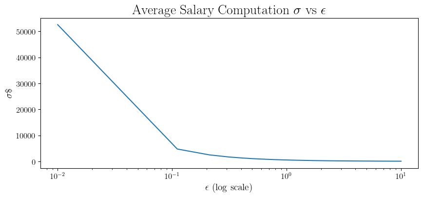
For a better idea on the utility, looking at \(\varepsilon = 1/2\), \(\sigma\approx 806\). In turn, this means that: About 68% of the time, our reported average will be within \(806\) of the true mean. About 95% of the time, it will be within \(1,612\). Whether this is sufficient utility or not depends on the reason for computing the average, but it may be enough to get a decent idea about the average salary within a company.
The Gaussian Mechanism and Its Analysis
The process of adding Gaussian noise is usually called the Gaussian mechanism, which is an extremely fundamental building block of DP. First, we define the sensitivity of a function.
Definition: For a function \(f:\mathcal{D}\rightarrow \mathbb{R}^d\) computing a vector-valued statistic from a dataset, we define its sensitivity as
\(\Delta_f = \max_{D ,D':|D\triangle D'|=1} \|f(D) - f(D') \|_2\) where the condition \(|D\triangle D'|=1\) indicates that \(D\) and \(D'\) only differ by a single record.
Then, for a function \(f\) and a required \((\varepsilon,\delta)\)-DP level, based on the sensitivity \(\Delta_f\), the Gaussian mechanism calculates the needed \(\sigma\) and adds a noise drawn from \(\mathcal{N}(0, \sigma^2I)\) to the output of \(f\). Then, the Gaussian mechanism is simply
\[M(x) = f(x) + \mathcal{N}(0, \sigma^2I).\]For a simple version of the Gaussian mechanism, we may set \(\sigma = \frac{\Delta}{\varepsilon}\sqrt{2\ln(1/\delta)+2\varepsilon}\)
\(\begin{equation} L(M,D,D') \sim \mathcal{N}\left(\frac{\|f(D)-f(D')\|_2^2}{2\sigma^2}, \frac{\|f(D)-f(D')\|^2_2}{\sigma^2} \right) \end{equation}\) Finally, applying a tail bound on the Gaussian tail allows us to specify a sufficiently large \(\sigma\) so that \(P(L(M,D,D') > \varepsilon) \leq \delta.\) This then allows us to prove the \((\varepsilon, \delta)\) guarantee by key result 2.
While this value of \(\sigma\) is sufficient for (\(\varepsilon, \delta\))-DP, it is not necessary. In particular, the tail bound we applied during the proof may be loose for some values of \(\varepsilon\) and \(\delta\), resulting in a larger than needed \(\sigma\). For example, in the blog
Taking this one step further,
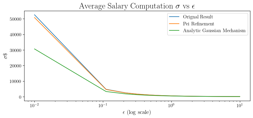
Taking another look at our example of computing the mean salary, we find out that for \(\varepsilon=0.5, \delta=10^{-6}\), we get \(\sigma\approx 1051\) with the original version, \(\sigma\approx 1026\) with Pei’s refinement, and \(\sigma\approx 806\) with the analytic version. Crucially, across all those values, we targeted the same privacy guarantee, just measured more tightly.
📝 The key takeaway message here and the reason we went into the details of the Gaussian mechanism is not to show the best way to implement the Gaussian mechanism. It is to illustrate that in DP:
- We really care about tighter bounds as: tighter bounds -> less noise -> more useful results for same privacy target
- In cases where it is possible to leverage numerical solvers to get tighter bounds, we are happy to do so.
The above two points are very important in both DP practice and research. While closed form bounds and asymptotics are useful in gaining intuition or proving the (non)optimality of some methods, most state-of-the-art DP implementations are attained using numerical solvers and numerous tricks to calibrate as tightly as possible the noise magnitude and compute the privacy guarantee.
From Gaussian Mechanism to DP-SGD
Privatizing Gradient Descent
Now that we introduced basic notions and tools of DP, let’s go back to our goal of training a neural network on a simple dataset, starting with the fundamental optimization algorithm in machine learning - gradient descent (GD). Given a dataset \(D = \{z_1,...,z_N\}\) and a model \(f_\theta\) parameterized by \(\theta\), GD aims to minimize the empirical loss \(R(f_\theta,D) = \sum_i R(f_\theta,z_i)\) through iterative updates:
Algorithm: Gradient Descent (GD)
- Input: Initial parameters $\theta_0$, Dataset $D := {z_1,…,z_N}$, learning rate $\eta$, number of steps $T$
- For \(t = 1\) to \(T\) do:
- Compute gradient: \(g_t = \frac{1}{N} \sum_{i\in[N]} \nabla_{\theta_{t-1}} R(f_{\theta_{t-1}},z_i)\)
- Update parameters: \(\theta_t = \theta_{t-1} - \eta g_t\)
- Output: \(\theta_T\)
Let’s first consider the simplest case: \(T=1\), i.e., we just want to take a single gradient step. The tools, which we have developed with the Gaussian mechanism, allow us to do this! To see how, let’s analyze the sensitivity of a single gradient computation after the initialization. We assume the adversary already knows \(\theta_0\). Then, our privacy depends on the only step accessing the data, i.e. our query function is: \(f(D) = \frac{1}{N} \sum_{i\in [N]} \nabla_{\theta_0} R(f_{\theta_0},x_i).\)
The challenge is that gradients could be arbitrarily large, making the sensitivity unbounded. However, we can fix this by clipping the individual gradients to a maximum \(\ell_2\) norm \(C\). This gives us \(f(D) = \frac{1}{N} \sum_{i\in [N]} \text{clip}_C(\nabla_{\theta_0} R(f_{\theta_0},z_i)),\)
where \(\text{clip}_C(x):={\min(1, C/\|x\|_2)}{x}\). This gives us bounded sensitivity of $2C/N$ for the averaged gradient. Now we can apply the Gaussian mechanism by adding an appropriately scaled Gaussian noise to make a single DP gradient step.
Algorithm: Private Gradient Descent (One Step)
- Input: \(\theta_0\), \(D\), learning rate \(\eta\), noise scale \(\sigma\), clip threshold $C$
- For each \(i\), compute: \(\tilde{g}_i = \text{clip}_C(\nabla R(f_{\theta_0},z_i))\)
- Average: \(\bar{g} = \frac{1}{N} \sum_i \tilde{g}_i\)
- Add noise: \(\hat{g} = \bar{g} + \mathcal{N}(0,(4\sigma^2C^2/N^2)I)\)
- Update: \(\theta_1 = \theta_0 - \eta\hat{g}\)
- Output: \(\theta_1\)
The Challenge of Multiple Steps: Adaptive Composition
In practice, training requires many gradient steps, a single gradient step gets us nowhere. Since each step accesses the data, we need to account for cumulative privacy loss through successive computations. In addition, each computation (gradient step) requires the output of the previous computation. What we showed in the previous subsection is that through clipping and noise addition, we are able to make a single gradient step satisfy DP. Thus, what we need is a method to calculate the $(\varepsilon_{\text{tot}}, \delta_{\text{tot}})$-DP guarantees of a mechanism, which works by combining and iteratively executing multiple \((\varepsilon, \delta)\) mechanisms. Let’s define this more formally:
Definition (Adaptive Composition): Let \(M_1,...,M_k\) be mechanisms where each \(M_i\) takes both dataset \(D\) and auxiliary input and the outputs of all previous mechanisms. Their adaptive composition is \(M_{[k]}(D):=(O_1, \ldots, O_k)\), where
- \(O_1 = M_1(D)\),
- \(O_2 = M_2(D,O_1)\),
- \(O_3 = M_3(D,O_1,O_2)\) and so on.

Let’s interpret how gradient descent with many steps fits within the adaptive composition framework. We set the $i$-th step of gradient descent as \(M_i\), taking the output of the previous gradient steps and accessing the data to compute the new parameters \(\theta_{i}\). Then, \(M_{[k]}\) is the mechanism that releases all the model checkpoints \(\theta_1,\ldots, \theta_k\)
- Training checkpoints are commonly saved for monitoring convergence, early stopping, ensembling
- Models may be fine-tuned from intermediate checkpoints
- In federated learning, updates are explicitly shared with all participating agents
Note that the notion of DP used in federated learning is usually slightly different than the one we are using. The guarantee is usually not with respect $D$ and $D'$ differing by one datapoint, but instead $D$ and $D'$ differ by all the datapoints belonging to a single user. This is well explained in .
Finally, going back to our goal of calculating \((\varepsilon_{\text{tot}}, \delta_{\text{tot}})\), we can achieve this using the advanced composition theorem:
Theorem (Advanced Composition)
: For \(\delta'\in (0,1)\), the \(k\)-fold adaptive composition of \((\varepsilon,\delta)\)-DP mechanisms satisfies \((\varepsilon',k\delta+\delta')\)-DP, where \(\varepsilon' = \varepsilon\sqrt{2k \ln(1/\delta')} + k\varepsilon(e^\varepsilon - 1)\) This is not tight. For the tight bound, check ..
A first try at DP training:
After introducing the advanced composition theorem, we technically have all the ingredients for a first trial to train a small two-layer neural network on a simple dataset. For our model we will use a simple two-layer neural network with ReLU activation and \(128\) hidden units. For the data, we will use \(5000\) randomly sampled images from MNIST. To train our model with DP, we first need to set the hyperparameters \(C\) (clipping norm) and \(T\) (number of iterations). Then, after picking the privacy guarantee we want by setting \(\varepsilon\) and \(\delta\), we can use the Gaussian mechanism along with advanced composition result to calculate the magnitude of Gaussian noise required at each iteration.
In fact, we may make use of a handy result from
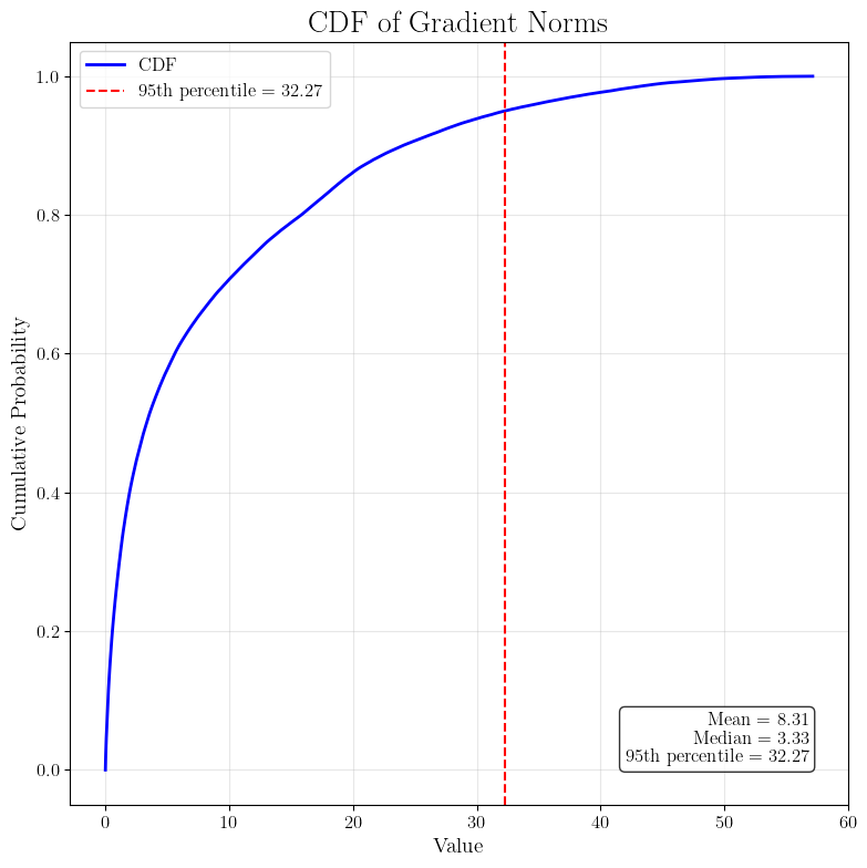
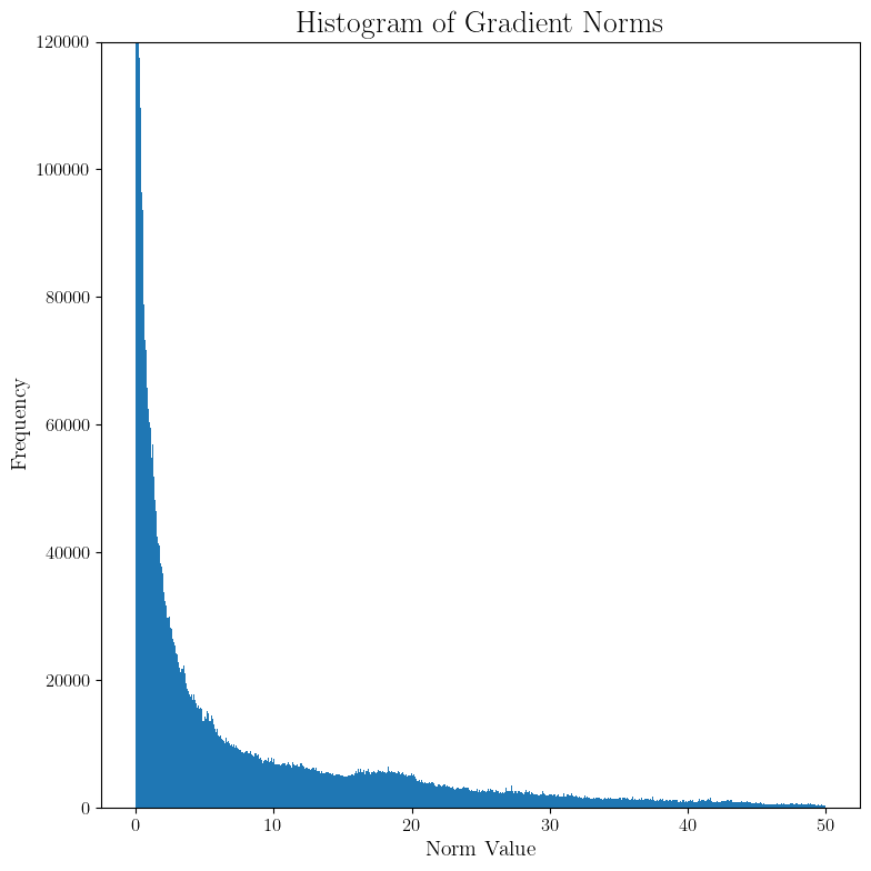
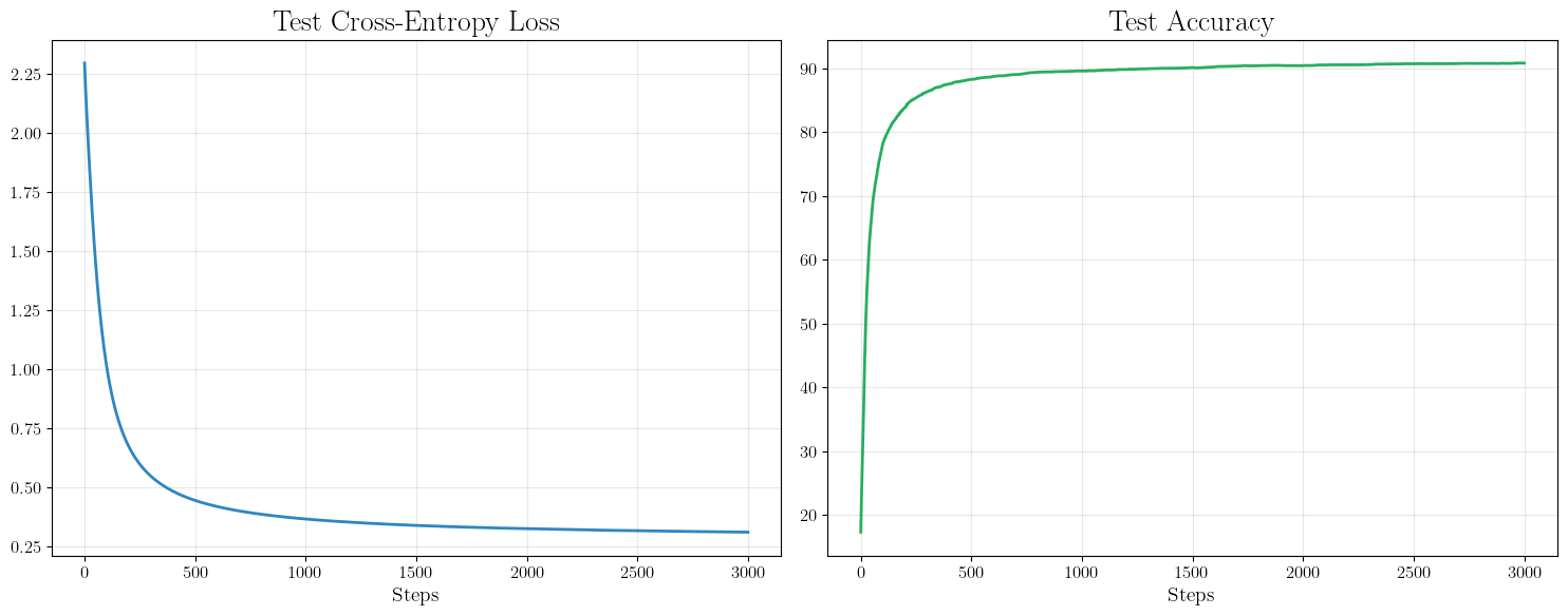
To get some intuition of the tuning of $C$ and $T$, let’s try a training run without any DP to see the gradient norms and the loss curves. We run gradient descent with learning rate $0.01$ for $5000$ iterations. For the gradients norm, the $95\%$ quantile is around $32$ and very small number of gradients go above $40$. For the sake of round numbers, let’s take $C=30$
Now let’s look at the test loss and accuracy. In the no DP setting, it looks like we should not train for more than $3000$ iterations. Also, very little progress occurs after $1000$.
Now, going back to our goal of DP training, depending on the number of iterations \(T\), let’s try to calculate the noise level \(\sigma\) needed for \(\varepsilon=1\), \(\delta=10^{-6}\), and \(C=30\).
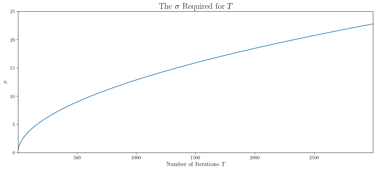
That’s actually a lot of noise to inject into GD. Let’s just try training for \(100\) iterations to see the current state of progress.
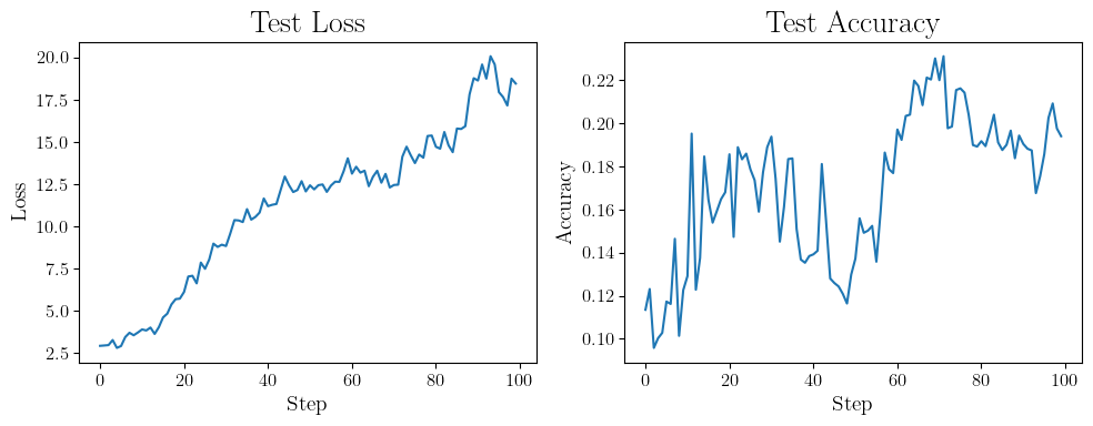
Well it’s not particularly good…
Tighter Analysis via Renyi Differential Privacy
Can we do better? Given that this blog exists, the answer is probably yes. The advanced composition theorem, while powerful, is mechanism-agnostic - it gives a worst-case bound that must hold for any sequence of \((\varepsilon,\delta)\)-DP mechanisms. For the Gaussian mechanism specifically, we can do much better.
Recall from our analysis of the Gaussian mechanism that the privacy loss random variable follows a Gaussian distribution:
\[L(M,D,D') \sim \mathcal{N}\left(\frac{\|f(D)-f(D')\|_2^2}{2\sigma^2}, \frac{\|f(D)-f(D')\|_2^2}{\sigma^2}\right)\]We also showed that to prove $(\varepsilon,\delta)$-DP, it suffices to bound the tails of this privacy loss random variable:
\[P(L(M,D,D') > \varepsilon) \leq \delta\]This suggests that if we can characterize the distribution of the privacy loss random variable more precisely, we might get tighter privacy guarantees. This leads us to Rényi Differential Privacy (RDP)
Definition: A mechanism \(M\) satisfies \((\alpha,\varepsilon)\)-RDP if for all neighboring datasets \(D,D'\): \(D_\alpha(M(D)||M(D')) := \frac{1}{\alpha-1}\log\mathbb{E}\left[\exp((\alpha-1)L(M,D,D'))\right] \leq \varepsilon\)
For the Gaussian mechanism with noise scale \(\sigma\Delta_f\), we can show that it satisfies \((\alpha,\frac{\alpha}{2\sigma^2})\)-RDP for all \(\alpha > 1\)
Theorem (RDP Conversion)
Thus, the parameter \(\alpha\) dictates the relation between \(\varepsilon\) and \(\delta\). This means that each moment bound on the privacy loss random variable captures a different tradeoff between \(\varepsilon\) and \(\delta\). Nonetheless, the key advantage of RDP is its much cleaner composition theorem:
Theorem (RDP Composition)
Thus to compose a series of RDP mechanisms, we can simply add their epsilons. The Gaussian mechanism has another remarkable property - it simultaneously satisfies RDP at all orders \(\alpha > 1\) with:
\[\varepsilon(\alpha) = \frac{\alpha}{2\sigma^2}.\]As a result, for any sequence of \(k\) Gaussian mechanisms with noise scale \(\sigma \Delta_f\), we achieve \((\alpha, \frac{k\alpha}{2\sigma^2})\)-RDP for all \(\alpha > 1\). Converting to \((\varepsilon,\delta)\)-DP, this gives us a family of guarantees:
\[\left(\frac{k\alpha}{2\sigma^2} + \frac{\log(1/\delta)}{\alpha-1}, \delta\right).\]For any choice of \(\alpha > 1\) and \(\delta > 0\). Different values of \(\alpha\) give us different tradeoffs - looking at the bound, larger \(\alpha\) values may work better for small \(\delta\).
The Gaussian mechanism satisfies RDP for an infinite list of alphas and that each \(\alpha\) gives rise to an infinite list of \((\varepsilon, \delta)\)-DP algorithms. A naturally arising question is: which \(\alpha\) should we pick. Again, the answer lies in leveraging automatic solvers to find the best possible \(\alpha\) for us. For example, if we want to calculate the DP privacy guarantee of the \(T\) times composition of the Gaussian mechanism, a typical workflow for using these automatic solvers is to give them the noise level \(\sigma\), the sensitivity \(\Delta_f\) of the function we are trying to make DP, and the number of times \(T\) we are composing this mechanism. Then, through a mixture of symbolic and numerical solutions, the solver will aim to find the best possible \(\varepsilon\) for a given \(\delta\) by trying a long list of candidate alphas. Another possible workflow is to give the solver the \(\varepsilon, \delta, \Delta_f\), and \(T\) and then to get the smallest possible \(\sigma\) needed. All of this in the hope of getting the tightest possible bounds. Thus, the theme of using numerical methods, which we first saw with the Analytic Gaussian mechanism, strikes back. Throughout this blog, we will be using the RDP accounting tools of Google dp-accounting library
A second try at DP training:
Armed with RDP and its cleaner composition result, let’s retry the experiments of the last subsection.
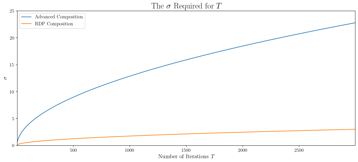
This is more encouraging. We need a way smaller noise for the same exact privacy guarantees. Let’s be brave and try training for \(T=200\) steps this time.
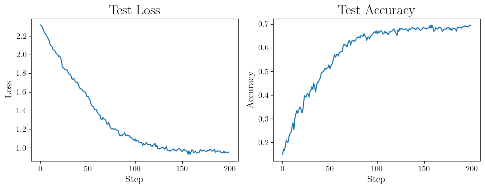
Well, we are actually able to train!
The Power of Subsampling: From GD to SGD
In practice, we rarely use full GD, preferring stochastic gradient descent (SGD), which operates on random minibatches. Beyond very small datasets on simple models, SGD is indispensable, as using the full dataset at each iteration is too computationally expensive. In particular, SGD subsamples a random minibatch at the start of each training iteration. However, a critical issue with subsampling is the expanded sensitivity. To illustrate, consider again the problem of computing the mean salary of \(n = 10^4\) employees, where the sensitivity of the full-dataset query scales as \(\mathcal{O}(1/n)\). Suppose instead of using the full dataset, we sample each employee independently with probability \(0.025\), sum the selected salaries, and normalize by \(250\) — the expected number of selected employees. In this case, the normalization is fixed, but the number of contributing salaries is random. The worst-case sensitivity now scales as \(\mathcal{O}(1/250)\), which is larger than in the full-dataset case. This increase in sensitivity forces us to add more noise to maintain the same privacy guarantee.
Nonetheless, implementing a differentially private SGD is still possible. Subsampling itself, under some conditions, can be shown to provide privacy benefits through privacy amplification by subsampling. Hence, the stochasticity of SGD makes each step more private, essentially allowing us to train with less noise. As a result, the tradeoff of increased sensitivity along with subsampling privacy amplification typically cancels out enabling us to use SGD
For the Gaussian mechanism specifically, when we combine:
- Poisson subsampling with rate \(q\)
- Gaussian noise with scale \(\sigma\Delta_f\)
We get the following RDP guarantee:
Theorem (Informal)
This \(O(q^2)\) factor is crucial as \(q\) is usually quite small in practice. Combined with RDP composition, this enables us to use much smaller noise for the same privacy guarantee.
Those building blocks allow us to finally recover the DP-SGD algorithm
- Randomly sample batch with rate \(q\)
- Clip the gradient for each example.
- Average and add \(\mathcal{N}(0,\sigma^2 I)\) noise
- Update parameters
- Track privacy via RDP composition
Technically the original DP-SGD was not introduced with the framework of RDP but with the moment accountant. Motivated by the structure of Gaussian noise, the authors proposed an algorithm to track the composition of Gaussian mechanisms through the moments of the privacy loss random variable. Later, RDP was introduced in , which in some sense generalized the approach of tracking composition through the moment behavior of the privacy loss random variable. For a nice discussion on this and a substantially more rigorous results on the amplification by subsampling of RDP, check . In an earlier work, Song et al. introduced a simpler version of DP-SGD
A third try at DP training.
The tight analysis through RDP and privacy amplification allows training SGD with reasonable noise scales. For example, let’s try to train for the previous setting with a subsampling rate \(q=0.05\).
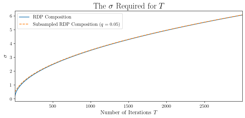
Using subsampling, we get basically the same noise levels for SGD as GD. However, it must be noted that the figures we have are also a function of the numerical solver we are using to compute the \(\sigma\) for a given setting. Here, as we previously stated, we are using the RDP accountant of the Google dp-accounting library. Using tighter numerical solvers, we can actually show that subsampling allows us to add less noise, especially at smaller values of \(T\) and \(q\).
Let’s try another training trial this time with SGD.
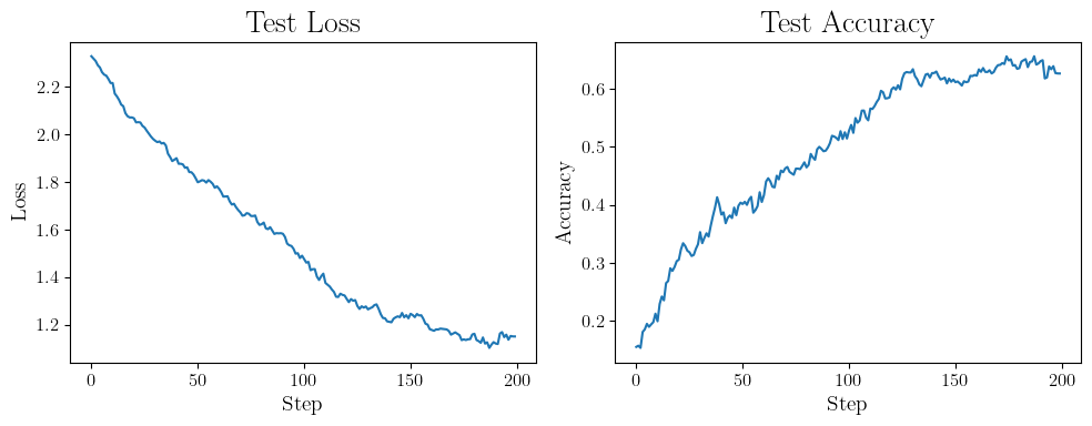
📝 In summary, in the previous subsection, we already showed that it is possible to effectively train DP neural networks using GD. Typically, due to computational requirements, we are forced to use SGD. However, in SGD, we are using smaller batches at each step and thus increasing the sensitivity. As a result, if we naively train with SGD, we will be forced to add much more noise at each step. Privacy amplification by subsampling allows us to solve this dilemma by showing that subsampling itself amplifies the privacy guarantee. So, when training with SGD, we need much less noise. All of these factors roughly even out, making the noise scale needed for DP-SGD reasonable.
Beyond DP-SGD: Using Correlated Noise
While DP-SGD with privacy amplification has become the standard approach for differentially private deep learning, it faces significant limitations:
-
Reliance on Privacy Amplification: Privacy amplification through subsampling requires strong assumptions on how data is processed. In many cases, the data may not fit in memory and sampling each datapoint with equal probability is not feasible.
-
Suboptimal Noise Addition: DP-SGD treats each gradient step independently, potentially leading noise accumulation. For the sake of illustration, consider the case where the gradients are constant. Then, the noise of DP-SGD, added independently at each iteration, will keep accumulating.
If not DP-SGD, what else can we do? Well, a growing line of work investigates adding correlated noise instead of independent noise at each iteration. To our knowledge, using this idea for training neural networks was first explored in
Putting Gradient Descent in Matrix Form
To understand the matrix factorization mechanism, let’s first look at how standard gradient descent can be viewed in matrix form. Consider training for \(T\) steps with learning rate \(\eta\). At each step \(t\), gradient descent computes:
\[\theta_t = \theta_{t-1} - \eta \nabla L_t(\theta_{t-1}).\]After \(T\) steps:
\[\theta_T = \theta_0 - \eta\sum_{t=1}^T \nabla L_t(\theta_{t-1}).\]This summation can be rewritten using matrices. Let’s stack all gradients into a matrix \(G\):
\[G = \begin{bmatrix} \nabla L_1(\theta_0) \\ \nabla L_2(\theta_1) \\ \vdots \\ \nabla L_T(\theta_{T-1})\end{bmatrix}.\]The parameter trajectory can then be written using a lower triangular matrix:
\[\begin{bmatrix} \theta_1 \\ \theta_2 \\ \vdots \\ \theta_T \end{bmatrix} = \begin{bmatrix} \theta_0 \\ \theta_0 \\ \vdots \\ \theta_0 \end{bmatrix} - \eta\begin{bmatrix} 1 & 0 & \cdots & 0 \\ 1 & 1 & \cdots & 0 \\ \vdots & \vdots & \ddots & \vdots \\ 1 & 1 & \cdots & 1 \end{bmatrix} \begin{bmatrix} \nabla L_1(\theta_0) \\ \nabla L_2(\theta_1) \\ \vdots \\ \nabla L_T(\theta_{T-1}) \end{bmatrix}.\]Let’s denote this lower triangular matrix by \(A\), i.e.,
\[A := \begin{bmatrix} 1 & 0 & \cdots & 0 \\ 1 & 1 & \cdots & 0 \\ \vdots & \vdots & \ddots & \vdots \\ 1 & 1 & \cdots & 1 \end{bmatrix}.\]Then we can write all iterations of gradient descent in a more compact form
\[\Theta = \Theta_0 - \eta AG,\]such that \(\Theta_0\) is the matrix with all rows set to \(\theta_0\) and the \(i\)-th row of \(\Theta\) is \(\theta_i\). Here, \(A\) encodes how past gradients influence current parameters. Each row of \(A\) represents which gradients have been accumulated up to that step.
DP-SGD in Matrix Form
Now, let’s consider DP-SGD, which adds noise at each step:
\[\theta_t = \theta_{t-1} - \eta(h_t + z_t)\]where \(z_t \sim \mathcal{N}(0, \sigma^2I)\) and \(h_t\) is the stochastic clipped gradient at iteration \(t\). Again, we can write in a more vectorized form, as
\[\begin{bmatrix} \theta_1 \\ \theta_2 \\ \vdots \\ \theta_T \end{bmatrix} = \begin{bmatrix} \theta_0 \\ \theta_0 \\ \vdots \\ \theta_0 \end{bmatrix} - \eta A \left(\begin{bmatrix}h_1\\ h_2 \\ \vdots \\ h_T \end{bmatrix} + \begin{bmatrix} z_1 \\ z_2 \\ \vdots \\ z_T \end{bmatrix}\right).\]Alternatively, we may also express this in the more compact form as \(\Theta = \Theta_0 - \eta A(H + Z)\) with matrix \(Z\) being the stacking of all noise vectors.
One drawback of DP-SGD is independent noise accumulation. To see why correlating noise across steps could help, let’s analyze how noise accumulates in DP-SGD versus alternative schemes. Consider a simple case where we make two steps, then
\[\theta_2 = \theta_0 - \eta(h_1 + z_1) - \eta(h_2 + z_2).\]Since \(z_1\) and \(z_2\) are independent, the total noise variance is \(2\eta^2\sigma^2\). More generally, after \(k\) passes, the variance grows linearly with \(k\). Now consider an alternative scheme where \(z_1 = -z_2\), then \(\theta_2 = \theta_0 - \eta(h_1 + h_1)\)
The noise cancels out. However, releasing \(\theta_2\) clearly offers no privacy guarantees at all. While this specific scheme isn’t DP, it illustrates how correlating noise across steps that process the same data could reduce total variance. Then, the question becomes how to do so in a DP way.
The Matrix Factorization Framework
Let’s try to generalize and take a wider perspective on DP-SGD. From writing it in matrix form, we can understand DP-SGD as a method to compute \(AH\) in a DP way by outputting
\[\widehat{AH} = A(H+Z),\]with a noise matrix \(Z\). The key insight is that we can factorize \(A = BC\). Again, our goal is still to report a DP version of \(AH\). However, we can now do it in an alternative way by using
\[\widehat{AH} = B(CH+Z).\]Here, we shift the placement of the DP mechanism to make it on the computation of \(CH\). Since \(A\) is independent of the data, \(B\) is also independent of the data. So if \(CH\) is computed in a DP way, then so will \(BCH=AH\). Then, if \(C\) is invertible, we can equivalently rewrite this as
\[\widehat{AH} = A(H+C^{-1}Z).\]This is actually what we want as the noise: the matrix \(C^{-1}Z\) is made from correlated noise. Assuming we factorize \(A=BC\) with \(B=A\) and \(C=I\). Then, the above statement reduces to
\[\widehat{AH} = A(H+C^{-1}Z) = AH+AZ.\]This is how DP-SGD works, as for our application, the \(i\)-th row of \(H\) is the \(i\)-th gradient vector. In addition, each row of \(Z\) is an independent realization from \(\mathcal{N}(0,\sigma^2 I)\). If we want to add correlated noise, we need to have \(C^{-1}\neq I\). Now, the question is finding a factorization \(A=BC\) such that
- \(C\) is invertible
- \(C^{-1}\) has a noise correlation structure that makes as much as possible of the total noise cancel out, in other words, optimizes the utility result.
- Evaluate the needed scale \(\sigma\) of the noise \(Z\), such that \(CH+Z\), or equivalently, \(H+C^{-1}Z\) is \((\varepsilon,\delta)\)-DP
In other words, various choices of \((C, \sigma)\) can be made to ensure \((\varepsilon,\delta)\)-DP, and some result in a better utility than the one choice \(C=I\).
Finding \(B\) and \(C\) to achieve the above goals is non-trivial. Again, we strongly rely on numerical solvers to find the best \(B\) and \(C\) and correspondingly calculate the required \(\sigma\) for \((\varepsilon, \delta)\)-DP. For details, refer to
- Be careful how you sample: we used Poisson sampling for DP-SGD, i.e., at each iteration, each datapoint is randomly selected with some fixed probability. We need to be careful how we sample datapoints with the matrix factorization setting. You cannot just plug the Poisson subsampling. In particular, when computing \((\varepsilon, \delta)\) guarantees, we must account for the maximum number of times any datapoint is used in gradient computations and a sampling structure where a datapoint cannot participate in gradient computations less than a prespecified fixed number of steps apart. Violating either will invalidate the privacy analysis.
- Subsampling amplification: one advantage of matrix factorization is that it is competitive with DP-SGD even without fully relying on any privacy amplification through subsampling
. A privacy amplification through subsampling for the matrix factorization was introduced in . With this amplification, in the settings tested in the paper, the matrix factorization mechanism was always Pareto optimal with respect to the privacy-accuracy tradeoff. Again, one should be careful with subsampling amplifications as they should be implemented in a way that does not violate the previous remark.
Structure of \(B\) and \(C\).
To illustrate a possible structure of the matrices \(B\) and \(C\), we use the matrices computed and released by

Note that we strongly care about the structure of \(C^{-1}\) as it modulates the correlation between the noise added at different iterations. Thus, let’s plot the distribution of the elements in \(C^{-1}\).
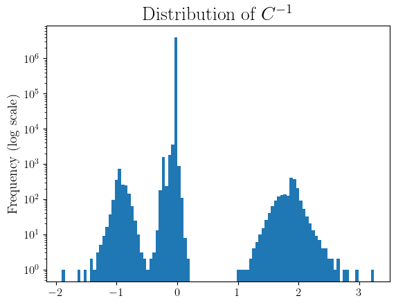
While most elements are zero, we can observe a positive and a negative cluster. The negative cluster allows for negative correlation between noise added at different iterations, which causes some of the noise to cancel out. Specifically, returning to our optimization setting, at iteration \(i\), the output of our mechanism is
\[\theta_i = \theta_0 - \eta A_{[i,:]}(H+C^{-1}Z),\]where \(A_{[i,:]}\) is the \(i\)-th row of \(A\). Thus, the standard deviation of the noise at iteration \(i\) can be seen as scaled with \((AC^{-1})_{[i,:]}\). To illustrate the benefit of using a noise correlation matrix, i.e, \(C\neq I\), we can plot the \(\ell_1\) norms of \((AC^{-1})_{[i,:]}\) and \(A_{[i,:]}\) across iterations.
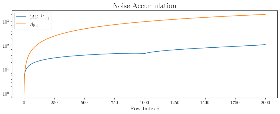
We can see that the curve corresponding to \(A_{[i,:]}\) increases at a much higher rate as none of the noise cancels out.
A fourth try at DP training
Now let’s go back to the running MNIST training setting, where we train a two-layer neural network on a \(5000\) images of MNIST with \((\varepsilon, \delta)\)-DP for \(\varepsilon=1\) and \(\delta=1e-6\). For the matrices \(B\) and \(C\) and the calibration of \(\sigma\), we used the tools released by
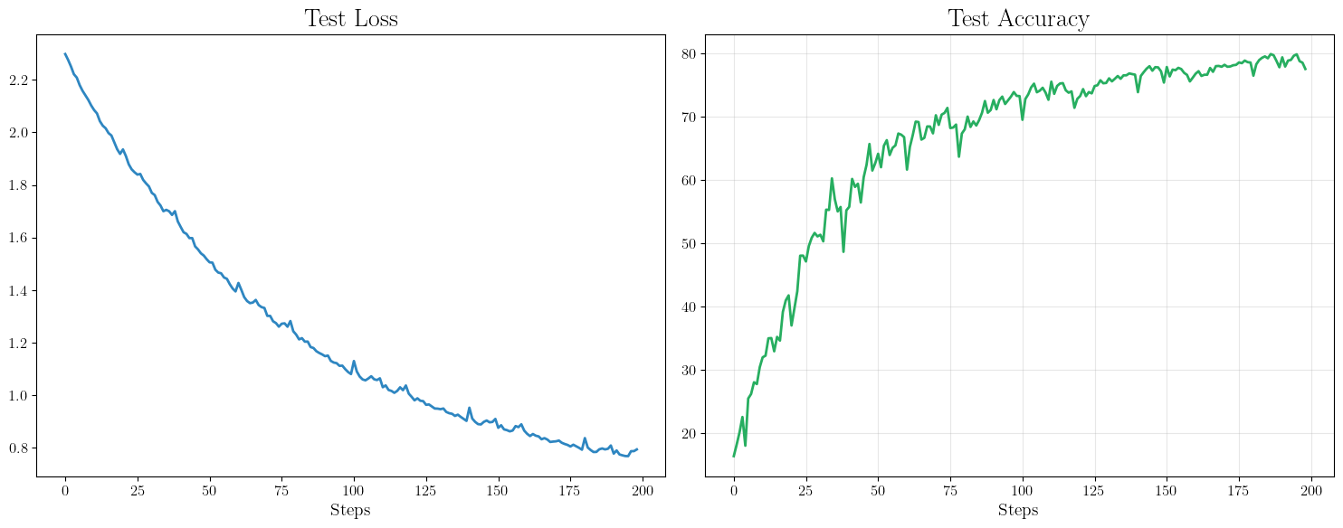
This is competitive with DP-SGD.
Conclusion
In this blog post, we explored the building blocks of differentially private training through two main approaches:
- DP-SGD, which adds independent Gaussian noise at each iteration, with privacy amplification through subsampling
- Matrix factorization mechanisms, which reduce noise accumulation by using carefully correlated noise across iterations
Both approaches offer viable paths to private deep learning, with different tradeoffs. For practitioners looking to train neural networks with differential privacy, experimenting with both approaches may be valuable, as their relative performance can depend on factors like model architecture, dataset size, and privacy requirements.
Finally, we added some of the code to generate the simulations in this repo, which will also host any post-publication updates or corrections to the blog.
Acknowledgments
We are deeply grateful for the insightful feedback and suggestions that helped shape and improve this blog post. We extend our sincere thanks to the anonymous reviewers for their valuable comments. We would also like to express our appreciation to Paul Mangold, Edwidge Cyffers, Adrien Majka, Martin Van Waerebeke, Daniel Berg Thomsen, and Renaud Gaucher for their careful reading and constructive feedback during the preparation of this work.