Unraveling The Impact of Training Samples
How do we quantify the influence of datasets? Recent works on Data Attribution Methods shed light on this problem. In this blog post, we introduce Data Attribution Methods which leverage robust statistics and surrogate functions, and present their applications like distinguishing the feature selection difference of learning algorithms, detecting data leakage, and assessing model robustness.
How do we quantify the true influence of datasets? What role does the influence score play in refining datasets and unraveling the intricacies of learning algorithms? Recent works on Data Attribution Methods give us an interesting answer to these problems.
This blog post revisits several proposed Data Attribution Methods which aim to quantitatively measure the importance of each training sample with respect to the model’s output. The blog post also demonstrates the utility of the data attribution methods by providing some usage examples, e.g. understanding the difference of learning algorithms, checking data leakage, and analyzing the model robustness .

Motivation of data attribution. For a given target, we want to quantify the influence of each of the training samples. Therefore, it’s more interpretable for us to understand model decisions and bias.
Data Attribution Methods
Exploring various milestone frameworks offers valuable insight into understanding the impact of training samples. Let’s delve into some established methods used for data attribution.
Influence Functions
In the paper Understanding Black-box Predictions via Influence Functions
The intuition behind the influence function is by looking at the difference of test loss after one training sample removal or perturbation. The calculation is given as follows:
\[\mathcal{I}_{\text{removal,loss}}(z,z_{\text{test}}):=\frac{dL(z_\text{test},\hat\theta_{\epsilon,z})}{d\epsilon}\Bigg|_{\epsilon=0}\approx-\nabla_\theta L(z_{\text{test}},\hat\theta)^\top H_{\hat\theta}^{-1}\nabla_\theta L(z,\hat\theta)\]Show algorithm step by step
Given the assumption we made, our algorithm can find the optimal $\hat\theta$ which minimizes the empirical risk and also guarantees the existence of the positive definite Hessian matrix: $$R(\theta):=\frac{1}{n}\sum L(z_i,\theta), \ \ \hat\theta=\arg\min_\theta R(\theta)$$ $$H_{\hat\theta}:=\frac{1}{n}\sum \nabla _\theta^2 L(z_i,\hat\theta).$$ Given the intuition written above, we look at the parameter difference $\Delta_\epsilon=\hat\theta_{\epsilon, z}-\hat\theta$ by perturbing one training sample: $$\hat\theta_{\epsilon, z}=\arg\min_{\theta}\{R(\theta)+\epsilon L(z,\theta)\}$$ Recall our goal is to estimate how does the algorithm changes with sample perturbation, we can express our goal as $\frac{d \hat\theta_{\epsilon, z}}{d \epsilon}$. Since $\hat\theta_{\epsilon, z}$ is a minimizer of the pertured loss. We can write its first order optimality condition: $$0=\nabla R(\hat\theta_{\epsilon, z})+\epsilon \nabla L(z,\hat\theta_{\epsilon, z}).$$ By performing a taylor expansion on $\hat\theta_{\epsilon, z}$, we can estimate $$0\approx \left[ \nabla R(\hat\theta)+\epsilon \nabla L(z,\hat\theta)\right] + \left[ \nabla^2 R(\hat\theta)+\epsilon \nabla^2 L(z,\hat\theta)\right]\Delta_\epsilon.$$ Since $\hat\theta$ minimizes $R$ and $o(\epsilon)$ term can be omitted, we can solve for $\Delta_\epsilon$ as follows: $$\Delta_\epsilon\approx -\nabla^2 R(\hat\theta)^{-1} \nabla L(z,\hat\theta)\epsilon \Rightarrow \frac{d \Delta_\epsilon}{d \epsilon}\Bigg|_{\epsilon=0}=\frac{d \hat\theta_{\epsilon,z}}{d\epsilon}\Bigg|_{\epsilon=0}=-H_{\hat\theta}^{-1}\nabla_\theta L(z,\hat\theta) $$
Therefore, $\mathcal{I}_{\text{removal,loss}}(z,z_{\text{test}}):=\frac{dL(z_\text{test},\hat\theta_{\epsilon,z})}{d\epsilon}\Bigg|_{\epsilon=0} =\frac{dL(z_\text{test},\hat\theta_{\epsilon,z})}{d\hat\theta_{\epsilon,z}}\frac{d \hat\theta_{\epsilon,z}}{d\epsilon}\Bigg|_{\epsilon=0}\approx-\nabla_\theta L(z_{\text{test}},\hat\theta)^\top H_{\hat\theta}^{-1}\nabla_\theta L(z,\hat\theta)$
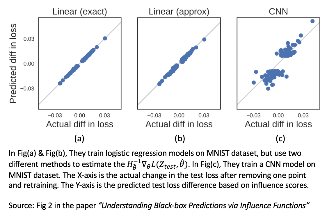
Since one training sample removal can be understood as setting $\epsilon=-\frac{1}{n}$, we can predict the corresponding test loss difference by $-\frac{1}{n}\mathcal{I_{\; remove, loss}} \;(\mathcal{z}, \mathcal{z}_{\text{test}})$. By comparing the predicted test loss difference and the actual test loss difference by leave-one-out retraining, we can verify the accuracy of the proposed influence scores, as shown in the figure below.

Based on their experiments, we can empirically say that the proposed influence function performs well on the tasks which satisfy their underlying assumptions (the twice-differentiable and strictly convex assumption): In Fig(a) & Fig(b), under convex and convergent situations (Logistic Regression model & L-BGFS algorithm), the predicted loss difference and actual loss difference align well with each other. However, in Fig(c), under non-convex and non-convergent-guarantee situations(CNN model & SGD algorithm), the influence function could not make satisfying approximation.
Although the Influence Functions seem provide a good estimation of the importance of each training sample, the expensive computational cost on estimating Hessian matrix and the unstablility under non-convex and non-convergent-guarantee situations are big issues for this data attribution method.
Data Models
Another branch of methods for data attribution are sampling-based methods, such as the Datamodels work of Ilyas et al
How do we train such a linear surrogate function? Consider a fixed training dataset $S$, a learning algorithm $\mathcal{A}$, and a target example $z$, and a distribution $D_{S}$ over subsets of $S$. Use $D_S$ to repeatedly sample a number of $S_{i}$, train $f_{\mathcal{A}}(z; S_{i})$ using $\mathcal{A}$, and evaluating on $z$ to get pairs:
\[\{\Bigl(S_{1}, f_{\mathcal{A}}(z; S_{1})\Bigr),\cdot \cdot \cdot,\Bigl(S_{m}, f_{\mathcal{A}} (z; S_{m})\Bigr)\}\]A datamodel for a target example $z$ is a parametric function $g_w$ optimized to predict $f_{\mathcal{A}}(z; S_{i})$ from training subsets $S_{i}$, where $S_{i} \sim D_{S}$. The training objective is formulated as:
\[g_{w}: \{0, 1\}^{|S|} \mapsto \mathbb{R}, \text{ where }\; w = \underset{\beta}{argmin} \;\frac{1}{m}\sum_{i = 1}^{m}\mathcal{L}\Bigl(g_{\beta}(S_{i}),\; f_{\mathcal{A}}(z; S_{i})\Bigr) + \lambda||\beta||_{1}\]\(g_{w}(S_{i}) = <w, \mathbb{1}_{S_{i}}>\);
\(\mathcal{L}\bigl(g_{w}(S_{i}),\; f_{\mathcal{A}}(z; S_{i})\bigr) = \bigl(\;g_{w}(S_{i}) - f_{\mathcal{A}}(z; S_{i})\;\bigr)^2\);
\(f_{\mathcal{A}}(z; S_{i}):= (\text{logit for correct class}) - (\text{highest incorrect logit})\)
One Datamodel is specifically optimized to learn the data attribution of a fixed training dataset to a fixed but arbitrary example $z$. For a fixed sample of interest, we use $g_{w}$ to assign a learnable weight to each example in $S$. The sum of weights of all training example that’s included in $S_{i}$ is trained to predict the model outputs on $z$. This is formulated as the dot product between a weight vector $w$ and an indicator vector where entry $k$ indicates the existence of the $k^{th}$ training datapoint in $S$. Therefore, for a set of target examples, we can train a datamodel for each of them and construct a collection of datamodels.

Caption: Linear datamodels accurately predict true margins averaged across 100 models. Source: Fig 5 in the paper “Datamodels: Predicting Predictions from Training Data”
In their experiments using CIFAR-10, the authors reserved a specific subset of output pairs for evaluation. Here, $\alpha$ represents the subsampling fraction in relation to the training set size. For instance, in a training dataset with $|S| = 100$ data points, setting $\alpha = 0.2$ means each subset, $S_i$, comprises a fixed size of $|S_i| = 20$. They demonstrated that Datamodels effectively predict outcomes for unseen in-distribution test subsets. In the above plots, the bottom-right panel illustrates data for three color-coded random target examples, showing a strong Spearman correlation ($r > 0.99$) between predicted and actual outputs.
It’s crucial to note that the displayed margins represent averages across 100 models trained on $S_i$. This underscores a limitation of linear datamodeling:
achieving stability demands training a sufficient number of models for each subset. The figures from the original paper involves averaging over 100 models. When the true model output aren’t averaged across a significant number of models, it becomes apparent that the linearity is affected (see the figure below).

Despite the simplicity and accuracy of datamodels in predictions, training them for specific examples in large-scale scenarios poses challenges. Imagine training datamodels for ImageNet’s set of target examples, requiring training numerous models from scratch using ImageNet’s 1000-class training dataset. Ensuring stable prediction performance requires extensive computational resources, which is prohibitively expensive for modern foundation models.
TRAK
Inspired by Datamodeling framework and motivated to circumvent its expensive training cost, in TRAK:Attributing Model Behavior at Scale, Ilyas et al.
First, in this paper the authors further denote $\tau(z, S_i)$ as a data attribution method that assigns a real-valued score to each training input in $S_i$, indicating its importance to the model output $f_{\mathcal{A}}(z;S_i)$. The key concept of TRAK is to use first order Taylor expansion to approximate the trained model $\theta^{*}(S)$, of an algorithm for a given training dataset, and then use random projections to reduce the dimensionality of the gradient. Each time, we sample a training subset $S_i$ of size $\alpha \times |S|$ from $S$, and train a model $\theta^{*}(S_i)$, and then use random projection to project the high-dimensional gradient matrix at $\theta^{*}$ from $p$ to $k$ dimension where $k \ll p$. Ilyas et al.
$i$: the index of a training subset;
$\mathbf{Q}_{i}:=diag(1 - p_t^*)$ = $diag({(1 + exp(y_t \cdot f(z;\theta^{*})))^{-1}})$ where $p_t^*$ is the predicted correct-class probability at $\theta^{*}$;
> $t$: the index of a training sample in $S$;
$\mathbf{P}$: Random projection matrix that each entry is sample from a standard Gaussian distribution: $\mathbf{P}\sim \mathcal{N} (0, 1)^{p \times k}$ for $k \ll p$;
$\phi_{i}(z) = \mathbf{P}^T \nabla_{\theta} f(z;\theta^{*})$ a projected gradients from model $\theta^{*}(S_i)$ for target sample $z$;
$\Phi_{i} = [\phi_1 \cdot\cdot\cdot \phi_{m}]$ stacked projected gradients for all training data ${z_1,…z_m}$;
Further, TRAK samples $N$ training subsets of fixed size factor $\alpha$, trains each of them independently, and ensembles over these $N$ models: \(\tau_{TRAK}(z, S) := \mathfrak{S}((\frac{1}{N} \sum_{i=1}^{N} \mathbf{Q}_{i}) \cdot (\frac{1}{N} \sum_{i=1}^{N} \phi_{i}(z)^{T}(\Phi_{i}^{T}\Phi_{i})^{-1}\Phi_{i}^{T}), \hat{\lambda})\)
$\mathfrak{S}(\cdot; \lambda)$ is the soft thresholding operator;
$N$: total number of training subsets;
$m$: total number of training samples in $S$;
$\hat{\lambda}$ is the soft thresholding parameter, and it’s selected via cross-validation
Show algorithm step by step
Before introducing the implementation steps, Ilyas et al.
$x_t$ is an input in $\mathbb{R}^d$;
$y_t$ is the binary label;
$b_t$ the bias term
Then the authors further parametrize the learning algorithm with $\theta$ as the model parameters: $$\theta^{*}(S) := arg\; \underset{\theta}{min} \sum_{(x_t, y_t)\in S} log[1 + exp(-y_t \cdot (\theta^{T}x_t + b_t))]$$ Data attribution in binary logistic regression setting can be learned by using the _one-step Newton approximation_
$z$: target sample;
$f(z;\theta) :=\theta^{T}x+b$;
$z_t$: the $t^{th}$ training example, $z_t = (x_t, b_t, y_t)$;
$X \in \mathbb{R}^{n \times d}$ stacking all input in one matrix $X$;
$p_{t}^{*}:= (1 + exp(-y_t \cdot f(z_t; \theta^*)))^{-1}$
$p_{t}^{*}$ is the predicted correct-class probability at $\theta^{*}$;
$R$ is a diagonal $n \times n$ matrix with $R_{tt} = p_{t}\times (1-p_{t}^{*})$
Now that the Ilyas et al.
In this paper, the algorithm of TRAK is consist of five steps:
1. Linearizing the model output function via Taylor approximation, which reduces the model of interest to a linear funtion in parameter space. Consider $f(z;\theta)$ as a non-convex function, then we can approximate it with its Taylor expansion centered around $\theta^{\*}$:
$$\hat{f}(z;\theta):= f(z;\theta^{*}) + \nabla_{\theta} \; f(z;\theta^{*})^{T}(\theta - \theta^{*})$$ $$\theta^{*}(S) \approx arg\; \underset{\theta}{min} \sum_{z_t \in S} log[1 + exp(-y_t \cdot ( \underbrace{\nabla_{\theta} \; f(z;\theta^{*})^{T}}_{inputs}\;\theta + b_t))]$$ where
$f(z;\theta):=log(\frac{p(z;\theta)}{1 - p(z; \theta)})$
$b_t = f(z;\theta^{\*}) - \nabla_{\theta} \; f(z;\theta^{\*})^{T} \theta^{\*}$
2. Reducing the dimensionality of the linearized model using random projections. To preserve the model-relevent information, Ilyas et al
$\mathbf{P}\sim \mathcal{N} (0, 1)^{p \times k}$ for $k \ll p$
3. Estimating influences by adapting the one-step newton approximation.
$$\tau(z, S) := \phi(z)^{T}(\Phi^{T}\Phi)^{-1}\Phi^{T}\mathbf{Q}$$ where
$\mathbf{Q}:= diag(1 - p_{t}^*) = diag(\{(1 + exp(y_t \cdot f(z;\theta^{*})))^{-1}\})$;
$\mathbf{Q} \in \mathbb{R}^{n \times n}$ where each diagonal is a one minus correct-class probability term.
4. Ensembling over $N$ independently trained models. Each model is trained on a subset of the training set, $S_i \subset S$.
$$\tau_{N}(z, S) := (\frac{1}{N} \sum_{i=1}^{N} \mathbf{Q}_{i}) \cdot (\frac{1}{N} \sum_{i=1}^{N} \phi_{i}(z)^{T}(\Phi_{i}^{T}\Phi_{i})^{-1}\Phi_{i}^{T})$$
5. Inducing sparsity via soft-thresholding. $$\tau_{TRAK}(z, S) := \mathfrak{S}((\frac{1}{N} \sum_{i=1}^{N} \mathbf{Q}_{i}) \cdot (\frac{1}{N} \sum_{i=1}^{N} \phi_{i}(z)^{T}(\Phi_{i}^{T}\Phi_{i})^{-1}\Phi_{i}^{T}), \hat{\lambda})$$ where
$\mathfrak{S}(\cdot; \lambda)$ is the soft thresholding operator;
$\hat{\lambda}$ is the soft thresholding parameter, and it's selected via cross-validation

Caption: We trained 90 RestNet9 models independently on 90 randomly selected subsets of size factor 0.5 from $S$. Then we used TRAK to calculate influence score for the test dataset of CIFAR-10. These are two random samples that show the efficacy of TRAK. For the training images that have high TRAK scores, they are of the same category. While those of low TRAK scores are of different categories of the target image.

Ilyas et al.
In replicating the experiments detailed in Ilyas et al.
While TRAK offers an interpretable and computationally efficient way to analyze training data impact, its limitations cannot be overlooked. Further research is needed to propose better data attribution methods.
How do we use it?
Learning Algorithm Comparison
Data attribution methods estimate the importance of each training sample with respect to the model’s output. An natural idea comes up: can we leverage the data attribution methods to understand the learning algorithms’ difference based on how they weight the training data?
The paper ModelDiff: A Framework for Comparing Learning Algorithms
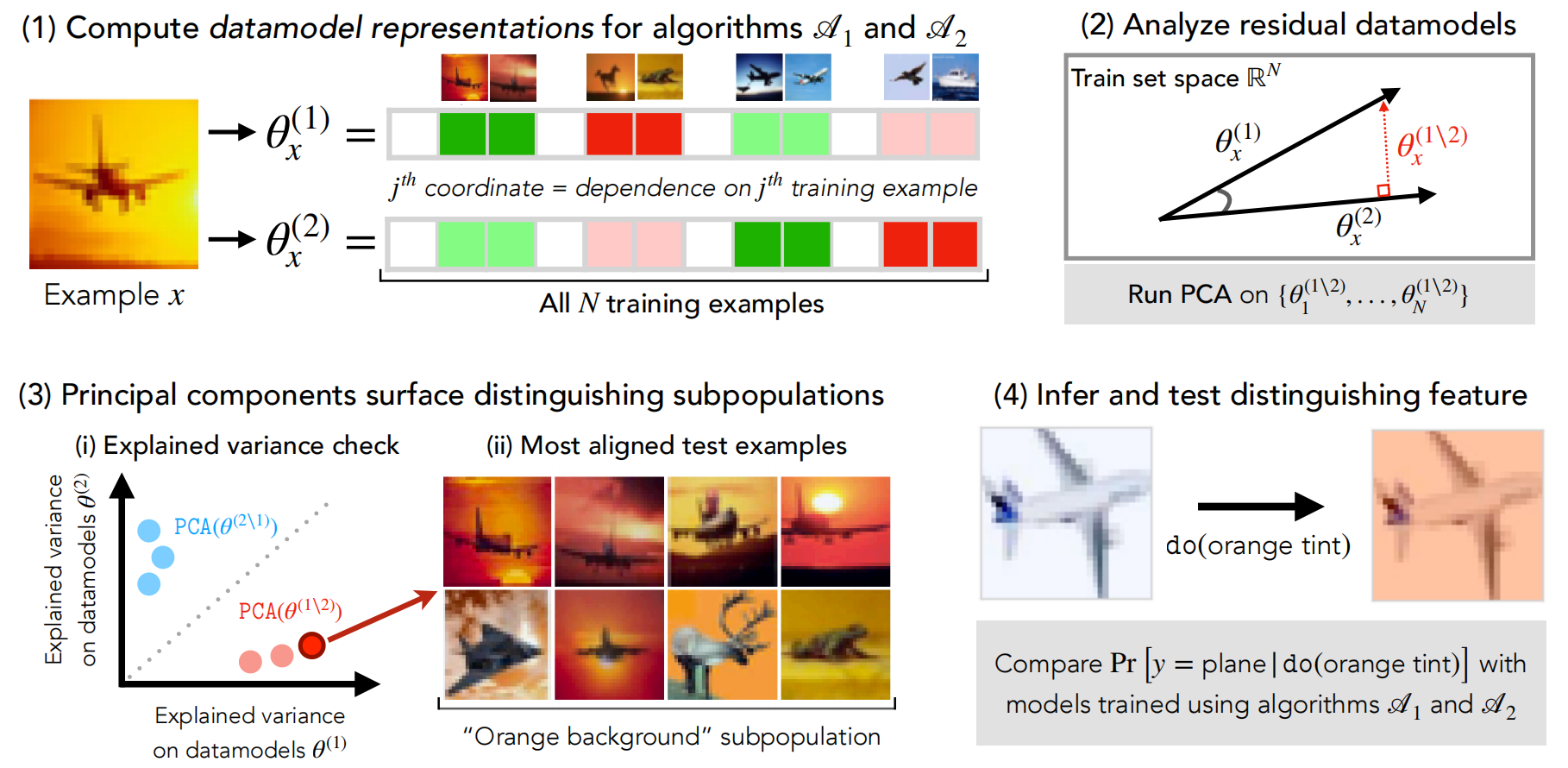
Therefore, we could get the importance matrix $\Theta^{|train | \times |test|}$ for each learning algorithm applied on a specific task. We apply matrix projection and PCA techniques on the importance matrix $\Theta$ to explore the distinguishing difference between how two algorithms use training samples. The detailed pipeline of comparing learning algorithm is depicted in the following figure.

Source: Figure 2 in the paper “MODELDIFF: A Framework for Comparing Learning Algorithms”
In the figure above, the authors PCA on the residual importance matrix (after projection, we remove the common importance allocation). The training samples corresponding to the TOP-K principal components (these principal component directions explain a significant amount of variance in one importance matrix but not the other) reflect the distinguishing subpopulations that one learning algorithm prefers, but another learning algorithm pays little attention to.
By visually checking these distinguishing subpolutations, we could speculate the semantic feature selection difference of two algorithms and then confirm it by applying the semantic feature transformations on test data and checking the model output difference.

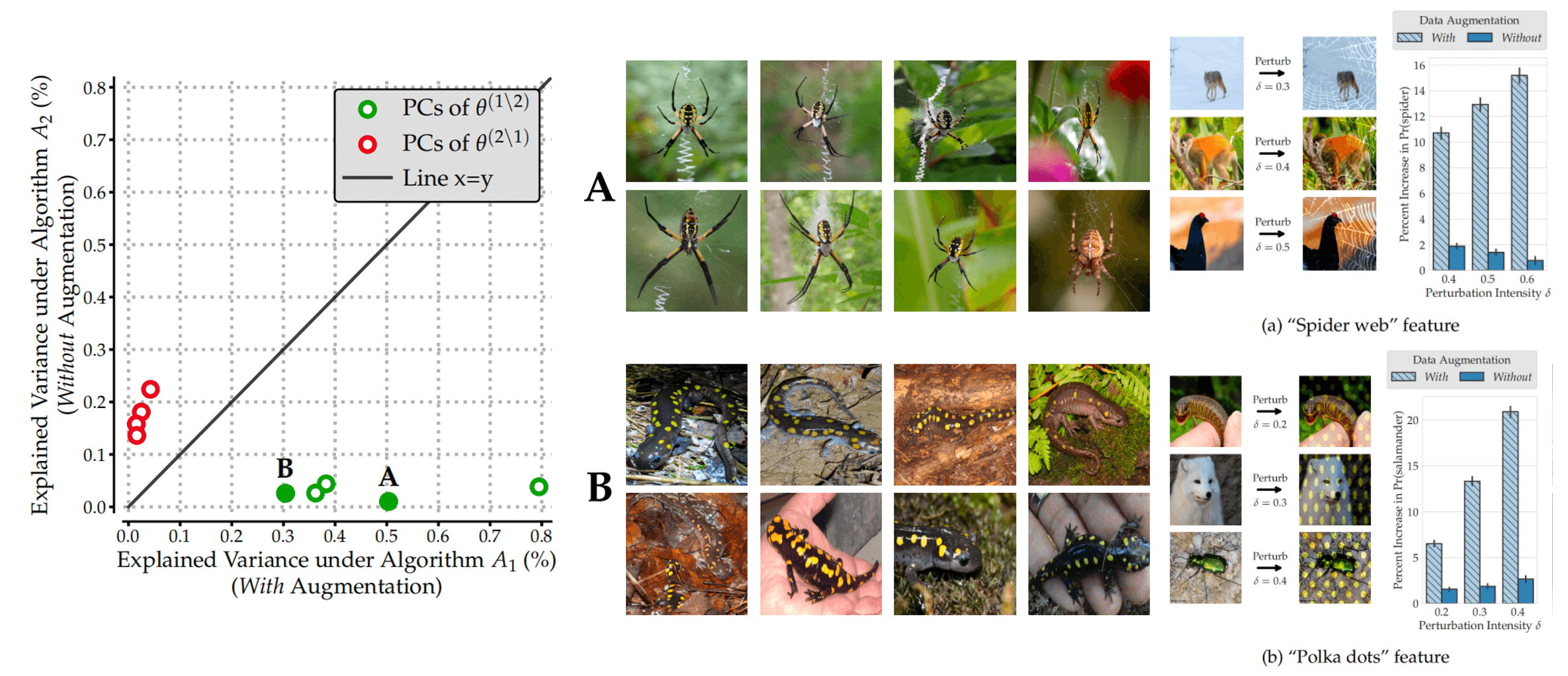
Source: Figure 3 in the paper “MODELDIFF: A Framework for Comparing Learning Algorithms”
For example, in the figure above, they compared two models trained on LIVING17 dataset. The only difference between these two models is whether they are trained with or without standard data augmentations. By exploring the training sample importance matrix using the method mentioned above, they speculated that the model trained with data augmentation prefers using “web” to predict the class “spider” and using “yellow polka dots” to predict the class “salamander”. Therefore, they added “web” or “yellow polka dots” texture to test samples and found out that only the prediction of the model with data augmentation changes a lot. This experiment verified the previous work that the data augmentation will enhance the texture bias.
The ModelDiff shows that the data attribution methods can be key tools for understanding model behaviors and distinguishing the subtle differences of algorithms.
Data Leakage Detection
Except for comparing learning algorithms, we can also leverage the importance score to find training samples which are most relevant to the model prediction. By empirically observing the training samples with different importance magnitude, Harshay et al.

_Source: Figure 3 in the paper “MODELDIFF: A Framework for Comparing Learning Algorithms”

Source: From the randomly selected validation points provided by Ilyas et al.
We can leverage such phenomenon to identify train-test leakage in different benchmark datasets. For example, in the second line of the figure, Harshay et al. identified significant data leakage on CIFAR10 dataset. Extending this data leakage detection technique to different datasets holds the potential to assist the ML community in curating datasets, thereby enhancing overall data quality.
Prediction Brittleness Examination
We can also use the data attribution methods to identify brittle predictions (i.e. the model outputs which are brittle to a few training samples removal) and estimate data counterfactual (i.e. the casual effect of removing a set of training samples on model outputs).
Specifically, we could leverage the sample importance scores to find the smallest training subset (defined as support set) such that removing them could flip the model prediction. By calculating the support set size for each test sample, we could know the brittleness of the model output with respect to the input.

Source: Fig 8 in the paper “Datamodels: Predicting Predictions from Training Data”
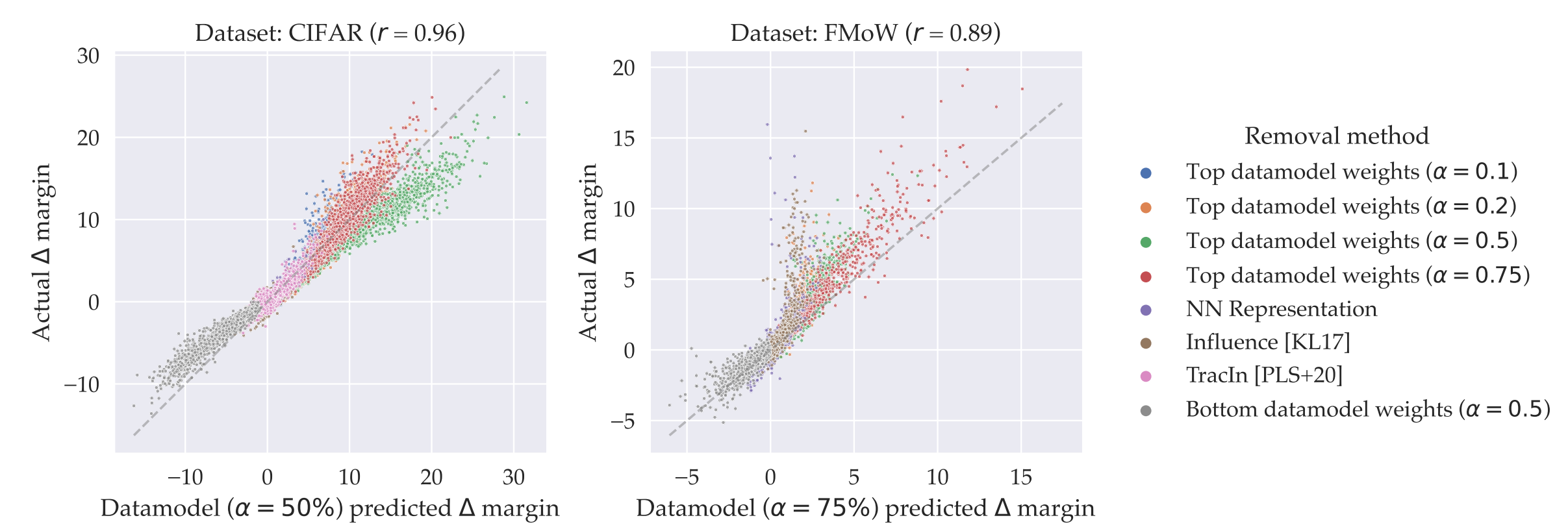
Another application involves data counterfactual estimation. As illustrated in the figure above, after the training subset removal, the observed changes in actual model logits closely align with the predicted model logits changes estimated through data attribution methods.
These experiments demonstrate that the data attribution methods could serve as efficient and convincing tools to investigate the sensitivity and robustness of the learning algorithms.
Conclusion
The data attribution methods give us an interesting answer to a natural question arising from the deep learning field: how does each training sample help with the model’s prediction? These methods can quantitatively measure the importance of each training sample with respect to the model’s output. The versatility of these methods extends across diverse applications, such as understanding learning algorithm behaviors, checking the data quality and analyzing the robustness of models.
Future works can focus on leveraging the data attribution methods to do dataset curation and model refinement. Also, investigating the scalability of the data attribution methods to larger datasets and different tasks remains a promising direction for enhancing their practical utility.