Understanding in-context learning in transformers

We propose a technical exploration of In-Context Learning (ICL) for linear regression tasks in transformer architectures. Focusing on the article Transformers Learn In-Context by Gradient Descent by J. von Oswald et al., published in ICML 2023 last year, we provide detailed explanations and illustrations of the mechanisms involved. We also contribute novel analyses on ICL, discuss recent developments and we point to open questions in this area of research.

What is in-context learning?

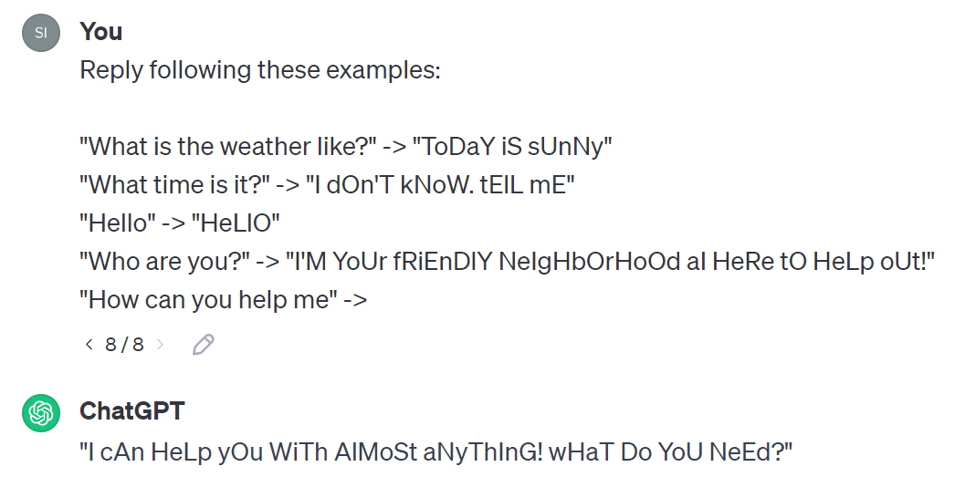
In-Context Learning (ICL) is the behavior first observed in Large Language Models (LLMs), whereby learning occurs from prompted data without modification of the weights of the model . It is a simple technique used daily and throughout the world by AI practitioners of all backgrounds, to improve generation quality and alignment of LLMs . ICL is important because it addresses full-on the once widespread criticism that for all their impressive performance, modern deep learning models are rigid systems that lack the ability to adapt quickly to novel tasks in dynamic settings - a hallmark of biological intelligence. By this new form of “learning during inference”, Large Language Models have shown that they can be, in some specific sense (once pretrained), surprisingly versatile and few-shot learners.

Figure 1: Example of a simple in-context prompt for ChatGPT.

Interestingly, it was around the release of GPT-2 and GPT-3 that researchers observed that an auto-regressive language model pre-trained on enough data with enough parameters was capable of performing arbitrary tasks without fine-tuning, by simply prompting the model with the task with few examples and letting it generate the output. In recent months, the research community has started to investigate the phenomenon of ICL in more details, and several papers have been published on the topic.

Figure 2: The number of papers published on the topic of ICL (and transformers) in the last years. Data extracted from arxiv.org on November 16th, 2023. In the last year alone, the number of papers on the topic has increased by more than 200%.

Specifically, since learning processes in biology and machine are often, if not always, understood in terms of iterative optimization, it is natural to ask what kind of iterative optimization is being realized during ICL, and how.

From large language models to regression tasks

Though ICL is generally regarded as a phenomenon exhibited by LLMs, we now hasten to study it in a non-language, small-scale model that enables more control and where ICL can still be shown to emerge. This simpler situation is that of a transformer model trained to regress a set of numerical data points presented in the prompt, with data points generated from a distinct function for each prompt, but where all prompts sample a function from the same general class (i.e. linear) at train and at test time. We will see that to some extent, this simplification allows for a mathematical treatment of ICL.

The following figure gives a visual representation of the ICL setup we will consider in this blog post. The model is a generic transformer pre-trained to solve generic linear regression tasks. At inference time, we can give the model a prompt with a new linear regression task, and it is able to solve it with surprisingly good performance.

Figure 3: The model is pre-trained to regress linear functions, and frozen during inference. With different context (input points), the model can still recover the exact underlying function. Use the slider to change the linear function to regress.

Objective of this blog post

The objective of this blog post is to understand how ICL is possible, and to present in an interactive way what is known of its underlying mechanism. Specifically, we will analyze the results reported in the paper Transformers Learn In-Context by Gradient Descent by J. von Oswald et al. recently published in ICML 2023 , which first showed that a simplified transformer model learns in-context by gradient descent. We will replicate the authors’ findings and then we will complement the discussion with a number of additional insights, before pointing to open questions. We hope the reader comes out of this post with a better vision of what fundamentally ICL is and the open challenges that remain.

Preliminaries and notations

First of all we need to agree on a mathematical formalization of in-context learning.

Before we start, let’s introduce some notation and color convention that will be used throughout the rest of the blog post. We will use the following colors to denote different quantities:

blue: inputs
green: model parameters
yellow: output

Vectors will be denoted with bold letters, e.g. \(\mba\), and matrices with bold capital letters, e.g. \(\mbA\). Additional notation will be introduced in-line when needed.

Formally, let’s define \(p(\mbx)\) as a probability distribution over inputs \(\mbx\in\cX\) and \(\cH\) a class of functions \(h: \cX \rightarrow \cY\). You can think of \(\cH\) as a set of functions that share some common properties, for example, the set of all linear functions, or the set of all functions that can be represented by a neural network with a given architecture. Also, let’s define \(p(h)\) as a probability measure over \(\cH\).

Figure 4: Visual representation of various parametric function classes (linear, sinusoidal, shallow neural network). Use the dropdown menu to select the function class.

Following the terminology of the LLM community, let’s define a prompt \(P\) of length \(C\) as a sequence of \(2C+1\) points \((\mbx_0, h(\mbx_0), \ldots, \mbx_{C-1}, h(\mbx_{C-1}), \mbx_{\text{query}})\) where inputs (\(\mbx_i\) and \(\mbx_{\text{query}}\)) are independently and identically drawn from \(p(\mbx)\), and \(h\) is drawn from \(\cH\). In short we will also write \(P_C = \left[\{\mbx_i, h(\mbx_i)\}_{i=0}^{C-1}, \mbx_\text{query}\right]\).

We posit that a model demonstrates in-context learning for a function class \(\cH\) if, for any function \(h \in\cH\), the model can effectively approximate \(h(\mbx_{\text{query}})\) for any new query input \(\textcolor{myblue}{\mbx}_{\text{query}}\). In other words, we say that a class of transformer models \(\cF\) learns in-context for a function class \(\cH\) if, for any \(\epsilon(C) > 0\), there exists a model \(f\in\cF\) such that the following inequality holds:

\[\begin{equation} \label{eq:in-context-error} \mathbb{E}_{\mbx,\mbx_{\text{query}}, \; h}\left[\ell\left(f(P_C), h\left(\mbx_{\text{query}}\right)\right) \right] \leq \epsilon(C), \end{equation}\]

where \(\ell\) is a loss function that measures the distance between the model output and the target function value, and the expectation is taken over \(p(\mbx)\) and the random choice of \(h\in\cH\) (the prompt \(P_C\) is constructed as described in the previous paragraph).

Note: The expectation in Equation \eqref{eq:in-context-error} is taken over the randomness of the input and the function. This means that we are considering the average performance of the model over all possible inputs and functions in \(\cH\).

Dataset construction and tokenization

For our setup, we will consider a linear regression problem, where the goal is to learn a linear function \(h_{\mbw}(\mbx) = \mbw^\top\mbx\), with \(\mbw\in\bbR^D\), from a set of in-context examples \(\{\mbx_i, \y_i\}_{i=0}^{C-1}\), where \(\mbx_i\in\bbR^D\) and \(\y_i\in\bbR\). So \(h_{\mbw} \in \cH\).

In order to better understand how the prompt is constructed starting from a regression task, let’s consider the following visual example:

Figure 5: Visualization of the data construction process, from the regression dataset, to the input prompt and the tokenization.

The figure shows a visual representation of the construction of a single input prompt. In particular, we first sample a weight \(\mbw\) from the distribution \(p(\mbw)\), and then we sample \(C\) inputs \(\mbx_i\) from \(p(\mbx)\), where \(C\) is the fixed context size. Finally, we compute the corresponding outputs \(\y_i = \mbw^\top\mbx_i\). We consider \(p(\mbx) = \cU(-1, 1)\), where \(\cU\) is the uniform distribution, and \(p(\mbw) = \cN(\mbzero, \alpha^2\mbI)\), where \(\cN\) is a multivariate Gaussian distribution of dimension \(D\), with \(0\) mean and \(\alpha\) standard deviation.

Defining \(c=C+1\) and \(d=D+1\), where \(C\) is the context size and \(D\) is the input dimension, we can represent the input as a matrix \(\mbE\in\bbR^{d\times c}\) (also referred to as token embeddings or, simply, embeddings), where the first \(C\) columns represent the context inputs \(\mbx_i\) and output \(\y\) and the last column represents the query input \(\mbx_{\text{query}}\) with \(0\) padding.

To construct a batch of regression problems, we just repeat the above procedure \(N\) times with the fixed context size \(C\), where \(N\) is the size of the batch.

A quick review of self-attention

In this section we will briefly review the self-attention mechanism, which is the core component of the transformer architecture .

Let \(\mbW^K, \mbW^Q \in \bbR^{d_k\times d}\), \(\mbW^V \in \bbR^{d_v\times d}\) and \(\mbW^P \in \bbR^{d \times d_v}\) the key, query, value and projection weight matrices respectively. Given an embedding \(\mbE\in\bbR^{d\times c}\), the softmax self-attention layer implements the following operation,

\[\begin{equation} \label{eq:softmax-self-attention} f_\text{attn} (\mbtheta_\text{attn}, \mbE) = \mbE + \mbW^P \mbW^V \mbE \sigma\left(\frac{(\mbW^K \mbE)^\top \mbW^Q \mbE}{\sqrt{d}}\right), \end{equation}\]

with \(\mbtheta_\text{attn}=\{\mbW^K, \mbW^Q, \mbW^V, \mbW^P\}\), where for simplicity we will consider \(d_k=d_v=d\), and \(\sigma(\cdot)\) is the softmax function applied column-wise. It’s simple to verify that the output dimension of \(f_\text{attn}\) is the same as the input dimension. To simplify further, we can also define the value, key and query matrices as \(\mbV = \mbW^V\mbE\), \(\mbK = \mbW^K\mbE\), \(\mbQ = \mbW^Q\mbE\), respectively.

Training details

Figure 6: Visualization of the pre-training process. The model is trained to minimize the loss function defined in Equation \eqref{eq:pre-train-loss-expectation}.

Once the dataset is created, we can train the model using the following objective:

\[\begin{equation} \label{eq:pre-train-loss-expectation} \cL(\mbtheta) = \mathbb{E}\left\|f\left(\mbtheta, \left[\{\mbx_i, \y_i\}_{i=0}^{C-1}, \mbx_\text{query}\right]\right) - \y_{\text{query}}\right\|^2, \end{equation}\]

where the expectation is taken over \(p(\mbx)\) and \(p(\mbw)\), with \(h_{\mbw}(\mbx) = \mbw^\top\mbx\). Note that the output of the model is a sequence of \(C+1\) values, i.e. same as the input prompt, and the loss is computed only on the last value of the sequence, which corresponds to the predicted query output \(\widehat\y_{\text{query}}\). Specifically, for reading out just the prediction for \(\mbx_{\text{query}}\), we multiply again by \(-1\) this last value. Note that this choice is completely transparent during model training, as it is equivalent to simply changing the sign of a few elements in the projection weight matrix \(\mbW^P\). The reason for this will be clear in the following sections. At each training iteration, we replace the expectation with an empirical average over a batch of \(N\) regression tasks, each made of a different set of context points \(\{\mbx_i^{(n)}, \y_i^{(n)}\}_{i=0}^{C-1}\), and a query input/target pain, \(\mbx^{(n)}_\text{query}\) and \(\y^{(n)}_{\text{query}}\), respectively. Note that because of the on-line creation of the dataset, during training the model will never see the same regression task twice.

Code for the transformer loss

This is the code for the loss computation, including the reading out of the query output.

Transformers can learn any linear function in-context

With all the preliminaries and notations in place, we can now start to analyze some results regarding the ability of transformers to learn linear functions in-context. One of the first papers that studied the ability of transformers to learn linear functions in-context is What Can Transformers Learn In-Context? A Case Study of Simple Function Classes by S. Garg et al . We will first replicate their results using a simpler configuration: using only up to 5 layers, single head attention, with 64 embedding units for a total number of parameters of 17K, 34K, 50K, 67K, 84K respectively.

In order to evaluate whether a model learns in-context for a given function class, we need to define a dataset of in-context examples. In this case we will only consider in-distribution test examples, i.e. examples that are drawn from the same distribution as the training examples.

In particular, we define the in-context test loss as:

\[\begin{equation} \label{eq:in-context-test-loss} \cL_\text{te}(\mbtheta) = \frac 1 N \sum_{n=0}^{N-1} \left\|f\left(\mbtheta, \left[\{\mbx_i^{(n)}, \y_i^{(n)}\}_{i=0}^{C-1}, \mbx^{(n)}_\text{query}\right]\right) - \y^{(n)}_{\text{query}}\right\|^2, \end{equation}\]

where we consider a fixed dataset of \(N=10000\) regression tasks, defined by a fixed set of in-context examples \(\{\mbx_i^{(n)}, \y_i^{(n)}\}_{i=0}^{C-1}\) and a query pair \(\mbx^{(n)}_{\text{query}}\) and \(\y^{(n)}_{\text{query}}\).

In the figure below, we report the in-context test loss (as defined in Equation \eqref{eq:in-context-test-loss}) for each model configuration, for various context sizes \(C\), from 2 to 100.

Figure 7: Transformers can learn linear functions in-context, reasonably well. The test loss decreases as the context size increases, and as the number of layers increases.

The experiment above shows that the test loss diminishes for larger context sizes, and also as the number of layers increases. These two main effects are clearly expected, as consequences of more data points and more compute, respectively, and they replicate the findings of Garg et al .

Linear self-attention is sufficient

From this point, we will depart from the classic softmax self-attention layer, and restrict our study to a linear self-attention layer, which is the setting considered in the paper of J. von Oswald et al . Recently, a number of papers have drawn connections between linear transformers and Fast Weight Programmers and have shown that linearized self-attention layers can be used to replace the softmax self-attention layer in transformers, with the advantage of reducing the computational complexity of the attention operation .

A linear self-attention updates embeddings \(\mbE\) as follows:

\[\begin{equation} f_\text{linattn} (\mbtheta_\text{linattn}, \mbE) = \mbE + \frac{\mbW^P \mbV\left(\mbK^\top \mbQ \right)}{\sqrt{d}}, \end{equation}\]

with \(\mbV, \mbK, \mbQ\) being the value, key and query defined right after Equation \eqref{eq:softmax-self-attention}.

Now, to analyze if a linear self-attention layer is sufficient to learn linear functions in-context, we can use the same experimental setup as before, but replacing the softmax self-attention layer with a linear self-attention layer.

Additionally, we also strip down the transformer to its bare minimum, i.e. we remove the normalization, the embedding layer, the feed-forward layer, and only use a single head. The only remaining component is the linear self-attention layer. Therefore, in the following we use the term “linear transformer” to refer to this simplified model.

Code for the linear transformer

This is the code for the linear transformer, without any normalization, embedding, etc with a single head

We test the linear transformer on the same dataset setup as before, and we will use the same number of layers as before, i.e. 1, 2, 3, 4, 5.

Figure 8: Linear transformers can also learn linear functions in-context, reasonably well. The test loss decreases as the context size increases, and as the number of layers increases.

What is special about linear self-attention?

From the previous section we have seen that a linear self-attention layer is sufficient to learn linear functions in-context. In this section we will try to understand why this is the case, starting from a review of least-squares regression and gradient descent.

Establishing a connection between gradient descent and data manipulation

In this section, we establish an important connection that will be fundamental to understand the mechanism behind ICL with linear self-attention. To do so we need to start from a simple linear regression problem, and we will show that we can achieve the same loss after one gradient step by changing the inputs and the targets, and keeping the weights fixed.

The loss for a linear regression problem is defined as: \(\begin{equation} \label{eq:linear-regression-loss} \cL_{\text{lin}}\left(\mbw, \{\mbx_i, {\y}_i\}_{i=0}^{C-1}\right) = \frac 1 {2C} \sum_{i=0}^{C-1} (\mbw^\top\mbx_i - \y_i)^2 \end{equation}\)

where \(\mbw\in\bbR^D\), \(\mbx_i\in\bbR^D\) and \(\y_i\in\bbR\). With a given learning rate \(\eta\), the gradient descent update is \(\mbw \leftarrow \mbw - \Delta \mbw\), where \(\begin{equation} \label{eq:linear-regression-gd-gradient} \Delta \mbw = \eta \nabla_{\mbw} \cL_{\text{lin}}\left(\mbw, \{\mbx_i, {\y}_i\}_{i=0}^{C-1}\right) = \frac{\eta}{C} \sum_{i=0}^{C-1} \left(\mbw^\top\mbx_i - \y_i\right)\mbx_i \end{equation}\) The corresponding loss (after the update) is: \(\begin{equation} \label{eq:linear-regression-loss-after-gd} \cL_{\text{lin}}\left(\mbw - \Delta \mbw, \{\mbx_i, {\y}_i\}_{i=0}^{C-1}\right) = \frac 1 {2C} \sum_{i=0}^{C-1} \left(\mbw^\top\mbx_i - \y_i - \Delta \mbw^\top\mbx_i\right)^2 \end{equation}\)

It is trivial to see that if we now define \(\widehat{\mbx}_i = \mbx_i\) and \(\widehat{\y}_i = \y_i + \Delta \mbw^\top\mbx_i\), we can compute Equation \eqref{eq:linear-regression-loss} with the new inputs and targets, i.e. \(\cL_{\text{lin}}(\mbw, \{\widehat{\mbx}_i, \widehat{\y}_i\}_{i=0}^{C-1})\), which is the same as the loss after the gradient descent update (Equation \eqref{eq:linear-regression-loss-after-gd}).

Building a linear transformer that implements a gradient descent step

As we just saw, the starting intuition is that we can build a gradient step on the linear regression loss by manipulating the inputs and the targets. This is the key insight of Oswald et al. that allows us to draw a connection between the gradient descent dynamics and the linear transformer.

Before stating the main result, recall the definitions of value, key and query as \(\mbV = \mbW^V\mbE\), \(\mbK = \mbW^K\mbE\), and \(\mbq_j = \mbW^Q\mbe_j\).

Main result: Given a 1-head linear attention layer and the tokens \(\mbe_j = (\mbx_j, \y_j)\), for \(j=0,\ldots,C-1\), we can construct key, query and value matrices \(\mbW^K, \mbW^Q, \mbW^V\) as well as the projection matrix \(\mbW^P\) such that a transformer step on every token \(\mbe_j \leftarrow (\mbx_i, \y_{i}) + \mbW^{P} \mbV \mbK^{T}\mbq_{j}\) is identical to the gradient-induced dynamics \(\mbe_j \leftarrow (\mbx_j, \y_j) + (0, -\Delta \mbW \mbx_j)\). For the query data \((\mbx_{\text{query}}, \y_{\text{query}})\), the dynamics are identical.

For notation, we will identify with \(\mbtheta_\text{GD}\) the set of parameters of the linear transformer that implements a gradient descent step.

Nonetheless, we can construct a linear self-attention layer that implements a gradient descent step and a possible construction is in block form, as follows.

\[\begin{align} \mbW^K = \mbW^Q = \left(\begin{array}{@{}c c@{}} \mbI_D & 0 \\ 0 & 0 \end{array}\right) \end{align}\]

with \(\mbI_D\) the identity matrix of size \(D\), and

\[\begin{align} \mbW^V = \left(\begin{array}{@{}c c@{}} 0 & 0 \\ \mbw_0^\top & -1 \end{array} \right) \end{align}\]

with \(\mbw_0 \in \bbR^{D}\) the weight vector of the linear model and \(\mbW^P = \frac{\eta}{C}\mbI_{d}\) with identity matrix of size \(d\).

If you are interested in the proof of construction for the GD-equivalent transformer, you can find it in the following collapsible section.

Proof of construction for the GD-equivalent transformer

To verify this, first remember that if \(\mbA\) is a matrix of size \(N\times M\) and \(\mbB\) is a matrix of size \(M\times P\),

\[\begin{align} \mbA\mbB = \sum_{i=1}^M \mba_i\otimes\mbb_{,i} \end{align}\]

where \(\mba_i \in \bbR^{N}\) is the \(i\)-th column of \(\mbA\), \(\mbb_{,i} \in \bbR^{P}\) is the \(i\)-th row of \(\mbB\), and \(\otimes\) is the outer product between two vectors.

It is easy to verify that with this construction we obtain the following dynamics

\[\begin{align} \left(\begin{array}{@{}c@{}} \mbx_j\\ \y_j \end{array}\right) \leftarrow & \left(\begin{array}{@{}c@{}} \mbx_j\\ \y_j \end{array}\right) + \mbW^{P} \mbV \mbK^{T}\mbq_{j} = \mbe_j + \frac{\eta}{C} \sum_{i={0}}^{C-1} \left(\begin{array}{@{}c c@{}} 0 & 0 \\ \mbw_0 & -1 \end{array} \right) \left(\begin{array}{@{}c@{}} \mbx_i\\ \y_i \end{array}\right) \otimes \left( \left(\begin{array}{@{}c c@{}} \mbI_D & 0 \\ 0 & 0 \end{array}\right) \left(\begin{array}{@{}c@{}} \mbx_i\\ \y_i \end{array}\right) \right) \left(\begin{array}{@{}c c@{}} \mbI_D & 0 \\ 0 & 0 \end{array}\right) \left(\begin{array}{@{}c@{}} \mbx_j\\ \y_j \end{array}\right)\\ &= \left(\begin{array}{@{}c@{}} \mbx_j\\ \y_j \end{array}\right) + \frac{\eta}{C} \sum_{i={0}}^{C-1} \left(\begin{array}{@{}c@{}} 0\\ \mbw_0^\top \mbx_i - \y_i \end{array}\right) \otimes \left(\begin{array}{@{}c@{}} \mbx_i\\ 0 \end{array}\right) \left(\begin{array}{@{}c@{}} \mbx_j\\ 0 \end{array}\right) = \left(\begin{array}{@{}c@{}} \mbx_j\\ \y_j \end{array}\right) + \left(\begin{array}{@{}c@{}} 0\\ - \frac{\eta}{C}\sum_{i=0}^{C-1} \left( \left(\mbw_0^\top\mbx_i - \y_i\right)\mbx_i\right)^\top \mbx_j \end{array}\right). \end{align}\]

Note that the update for the query token \((\mbx_{\text{query}}, \textcolor{output}{0})\) is identical to the update for the context tokens \((\mbx_j, \y_j)\) for \(j=0,\ldots,C-1\).

Experiments and analysis of the linear transformer

Now let’s do some experiments to verify the theoretical results. We will work within the same experimental setup as before with the same dataset construction, training procedure and testing procedure. In this first section, we consider a linear transformer with a single layer, and the transformer built as described in the previous section (the GD-equivalent transformer), i.e. with a linear self-attention layer that implements a gradient descent step.

During training, a linear transformer learns to implement a gradient descent step

We now study the evolution of the test loss of a linear transformer during training \(\cL(\mbtheta)\), and compare it to the loss of a transformer implementing a gradient descent step \(\cL(\mbtheta_\text{GD})\).

Figure 9: The loss of a trained linear transformer converges to the loss of a transformer implementing a gradient descent step on the least-squares regression loss with the same dataset. Use the slider to change the context size.

Although an empirical proof of such a functional equivalence would require to check the outputs for all possible test samples, we can try to gather more evidence by considering more closely the computations that unfold in the linear transformer during one pass.

To better understand the dynamics of the linear transformer, we now study the evolution of a few metrics during training (the L2 error for predictions, the L2 error for gradients and the cosine similarity between models).

Metrics details

The metrics introduced above are defined as follows:

L2 error (predictions) measures the difference between the predictions of the linear transformer and the predictions of the transformer implementing a gradient descent step and it is defined as \(\left\|f\left(\mbtheta, \left[\{\mbx_i, \y_i\}_{i=0}^{C-1}, \mbx_\text{query}\right]\right) - f\left(\mbtheta_\text{GD}, \left[\{\mbx_i, \y_i\}_{i=0}^{C-1}, \mbx_\text{query}\right]\right) \right\|^2\);
L2 error (gradients w.r.t. inputs) measures the difference between the gradients of the linear transformer and the gradients of the transformer implementing a gradient descent step and it is defined as \(\left\|\nabla_{\mbx_\text{query}} f\left(\mbtheta, \left[\{\mbx_i, \y_i\}_{i=0}^{C-1}, \mbx_\text{query}\right]\right) - \nabla_{\mbx_\text{query}} f\left(\mbtheta_\text{GD}, \left[\{\mbx_i, \y_i\}_{i=0}^{C-1}, \mbx_\text{query}\right]\right) \right\|^2\);
Model cosine similarity (gradients w.r.t. inputs) measures the cosine similarity between the gradients of the linear transformer and the gradients of the transformer implementing a gradient descent step and it is defined as \(\cos\left(\nabla_{\mbx_\text{query}} f\left(\mbtheta, \left[\{\mbx_i, \y_i\}_{i=0}^{C-1}, \mbx_\text{query}\right]\right), \nabla_{\mbx_\text{query}} f\left(\mbtheta_\text{GD}, \left[\{\mbx_i, \y_i\}_{i=0}^{C-1}, \mbx_\text{query}\right]\right)\right)\).

Figure 10: Comparison between the linear transformer and the GD-transformer during training. The predictions of the linear transformer converge to the predictions of the GD-transformer and the gradients of the linear transformer converge to the gradients of the GD-transformer. Use the slider to change the context size.

From this figure, we see that the predictions of the linear transformer converge to the predictions of the GD-transformer, and the gradients of the linear transformer converge to the gradients of the GD-transformer. Notably, this is true for all context sizes, though the convergence is faster for larger \(C\).

As a final visualization, we can also look at the evolution of the gradients of the linear transformer during training, as shown in the figure below. In this animation, we take six different regression tasks and we plot the gradients of the linear transformer during training and the exact gradients of the least-squares regression loss.

Figure 11: Animation of the gradients of the linear transformer during training. The loss landscape visualized is the least-squares regression loss (each task has its own loss). The gradients of the linear transformer are shown in red, while the gradients of the least-squares regression loss are shown in orange.

To reiterate, the loss landscape visualized is the least-squares regression loss and each task is a different linear regression problem with a different loss landscape. Once more, this is a visualization that the linear transformer is not learning a single regression model, but it is learning to solve a linear regression problem.

The effect of the GD learning rate

Next, we study the effect of the GD learning rate on the test loss of the GD-equivalent transformer. We believe this is an important point of discussion which was covered only briefly in the paper.

Indeed, this is the same procedure we have used to find the optimal GD learning rate for our previous experiments. We now show what happens if we use a different GD learning rate than the one found with line search. In the following experiment, we visualize this behavior, by plotting the metrics described above for different values of the GD learning rate.

Figure 12: Effect of the GD learning rate on the alignment between the linear transformer and the GD-transformer. The agreement between the two is maximized for a specific GD learning rate, which must be found by line search. Use the slider to manually change the GD learning rate.

Analytical derivation of the best GD learning rate

It turns out that having a line search to find the best GD learning rate is not necessary.

The analytical solution is provided below with its derivation reported in the collapsible section immediately following.

Analytical derivation of the best GD learning rate

We are interested in finding the optimal learning rate for the GD-transformer, which by construction (see main Proposition), is equivalent to finding the optimal GD learning rate for the least-squares regression problem. Consequently, the analysis can be constructed from the least-squares regression problem \eqref{eq:linear-regression-loss}.

Recall the GD update of the least-squares regression in \eqref{eq:linear-regression-gd-gradient} without taking into account of the learning rate. That is,

\[\begin{equation} \label{eq:linear-regression-gd-gradient-no-lr} \Delta \mbw = \nabla_{\mbw} \cL_{\text{lin}}\left(\mbw, \{\mbx_i, \y_i\}_{i=0}^{C-1}\right) = \frac{1}{C} \sum_{i=0}^{C-1} \left(\mbw^\top\mbx_i - \y_i\right)\mbx_i. \end{equation}\]

Now we consider the test loss of the least-squares regression defined as

\[\begin{equation} \cL_\mathrm{lin, te}(\{\mbw^{(n)}\}_{n=0}^{N-1}) = \frac{1}{N} \sum_{n=0}^{N-1} ((\mbx^{(n)}_\text{query})^\top \mbw^{(n)} - \y^{(n)}_\text{query})^2, \end{equation}\]

where \(N\) is the number of the queries, which is the same number of the regression tasks of the in-context test loss dataset. Similar to \eqref{eq:linear-regression-loss-after-gd}, after one step of the GD update \eqref{eq:linear-regression-gd-gradient-no-lr}, the corresponding test loss becomes

\[\begin{align} &\quad \ \ \cL_\mathrm{lin, te}(\{\mbw^{(n)} - \eta \Delta \mbw^{(n)}\}_{n=0}^{N-1}) \nonumber \\ &= \frac{1}{N} \sum_{n=0}^{N-1} \left((\mbx^{(n)}_\text{query})^\top (\mbw^{(n)} - \eta \Delta \mbw^{(n)}) - \y^{(n)}_\text{query}\right)^2 \nonumber \\ &= \frac{1}{N} \sum_{n=0}^{N-1} \left((\mbx^{(n)}_\text{query})^\top \mbw^{(n)} - \y^{(n)}_\text{query} - \eta (\mbx^{(n)}_\text{query})^\top \Delta \mbw^{(n)} \right)^2 \nonumber \\ &= \frac{\eta^2}{N} \sum_{n=0}^{N-1} ((\mbx^{(n)}_\text{query})^\top \Delta \mbw^{(n)})^2 + \cL_\mathrm{lin, te}(\{\mbw^{(n)}\}_{n=0}^{N-1}) \nonumber \\ &\quad \ - \frac{2\eta}{N} \sum_{n=0}^{N-1} ((\mbx^{(n)}_\text{query})^\top \mbw^{(n)} - \y^{(n)}_\text{query})(\mbx^{(n)}_\text{query})^\top \Delta \mbw^{(n)}. \label{eq:loss_query_W1} \end{align}\]

One can choose the optimum learning rate \(\eta^*\) such that \(\cL_\mathrm{lin, te}(\{\mbw^{(n)} - \eta \Delta \mbw^{(n)}\}_{n=0}^{N-1})\) achieves its minimum with respect to the learning rate \(\eta\). That is,

\[\begin{align} \eta^* \in \arg\min_{\eta > 0} \cL_\mathrm{lin, te}(\{\mbw^{(n)} - \eta \Delta \mbw^{(n)}\}_{n=0}^{N-1}). \end{align}\]

To obtain \(\eta^*\), it suffices to solve

\(\begin{align} \nabla_\eta \cL_\mathrm{lin, te}(\{\mbw^{(n)} - \eta \Delta \mbw^{(n)}\}_{n=0}^{N-1}) = 0. \end{align}\) From \eqref{eq:loss_query_W1} and plugging \(\Delta w^{(n)}\) in \eqref{eq:linear-regression-gd-gradient-no-lr}, we obtain \(\begin{align} \eta^* &= \frac{\sum_{n=0}^{N-1} ((\mbx^{(n)}_\text{query})^\top \mbw^{(n)} - \y^{(n)}_\text{query})(\mbx^{(n)}_\text{query})^\top \Delta \mbw^{(n)} } {\sum_{n=0}^{N-1} ((\mbx^{(n)}_\text{query})^\top \Delta \mbw^{(n)})^2} \nonumber \\ &= C \frac{\sum_{n=0}^{N-1} ((\mbx^{(n)}_\text{query})^\top \mbw^{(n)} - \y^{(n)}_\text{query}) \sum_{i=0}^{C-1} ((\mbw^{(n)})^\top \mbx_i^{(n)} - \y_i^{(n)})(\mbx_i^{(n)})^\top \mbx^{(n)}_\text{query}} {\sum_{n=0}^{N-1} \left( \sum_{i=0}^{C-1} ((\mbw^{(n)})^\top \mbx_i^{(n)} - \y_i^{(n)})(\mbx_i^{(n)})^\top \mbx^{(n)}_\text{query} \right)^2}. \end{align}\) Finally, for the initialization \(\mbw^{(n)} = 0\) for \(n = 0, \ldots, N-1\), the optimal learning rate can be simplified to be \(\begin{align} \eta^* = C \frac{\sum_{n=1}^{N-1} \y^{(n)}_\text{query} \left(\sum_{i=0}^{C-1}\left( \y^{(n)}_i{\left(\mbx^{(n)}_i\right)}^\top \mbx_\text{query}^{(n)}\right)\right) }{\sum_{n=1}^{N-1} \left(\sum_{i=0}^{C-1}\left(\y^{(n)}_i {\left(\mbx^{(n)}_i\right)}^\top \mbx_\text{query}^{(n)}\right)\right)^2}. \end{align}\)

Some comments on the analytical solution

This derivation of the optimal GD learning rate \(\eta^*\) agrees well with the line search procedure (up to the numerical precision of the line search procedure itself). While this is expected, let’s take a moment to understand why this is the case.

The analytical solution is obtained starting from the linear regression loss, while the line search procedure using the loss \(\cL(\mbtheta_\text{GD})\) defined in Equation \eqref{eq:pre-train-loss-expectation}. However, the two losses are equivalent by construction, hence the two procedures are equivalent.
Because the construction of the GD transformer is not unique, it’s not easy to see the effect of the GD learning rate once we compare it with the trained linear transformer. Recall that due to its parametrization, the linear transformer does not have an explicit \(\eta\) parameter, which it can be absorbed in any of the weight matrices in the linear self-attention layer. Yet, the linear transformer converges to the exact same loss of the GD-transformer for the optimal GD learning rate \(\eta^*\). This is expected because fundamentally the loss function used for the line search and the one used for the analytical solution is equivalent to the loss in Equation \eqref{eq:pre-train-loss-expectation} used during the transformer training.

Said differently, what we did in two steps for the GD-transformer (first build the \(\mbW^K, \mbW^Q, \mbW^V\) matrices, then find the optimal GD learning rate) is done implicitly during the training of the linear transformer.

The following table summarizes the three different procedures we have discussed so far.

	Loss function	GD learning rate
Least-squares regression	\(\cL_\text{lin}(\mbw-\Delta \mbw)\)	Explicit \(\eta^*\) by analytical solution
GD-transformer	\(\cL(\mbtheta_\text{GD})\)	Explicit \(\eta^*\) by line search
Linear transformer	\(\cL(\mbtheta)\)	Implicit \(\eta^*\) by training \(\mbtheta\)

Finally, one comment on the computational complexity of the two procedures. It doesn’t come as a surprise that the analytical solution is faster to compute than the line search: the line search requires on average 10 seconds to find the optimal GD learning rate, while the analytical solution requires only 10 milliseconds (both with JAX’s JIT compilation turned on, run on the same GPU).

If one layer is a GD step, what about multiple layers?

It is only natural to ask if the same behavior is observed for a linear transformer with multiple layers. In particular, if we take a trained linear transformer with a single layer (which we now know it implements a gradient descent step) and we repeat the same layer update multiple times recursively, will we observe the same behavior?

As we now show in the following experiment, the answer is no. In fact, the test loss for both the linear transformer and the transformer implementing a gradient descent step diverges as we increase the number of layers.

To stabilize this behavior, we use a dampening factor \(\lambda\), which is a scalar in \([0, 1]\), and we update the linear transformer as follows:

\[\begin{equation} \label{eq:linear-transformer-update} \mbE^{(l+1)} = \mbE^{(l)} + \lambda \mbW^P \mbV\left(\mbK^\top \mbQ \right), \end{equation}\]

where \(\mbE^{(l)}\) is the embedding matrix at layer \(l\), and \(\mbW^P, \mbV, \mbK, \mbQ\) are the projection, value, key and query matrices as defined before. Effectively, this is equivalent to applying a gradient descent step with scaled learning rate.

Code for the recurrent transformer

This is the code for the recurrent transformer, with a dampening factor \(\lambda\). Note that the attention layer is the same as before, but we now apply it multiple times.

Figure 13: A pre-trained transformer with a single layer can be used recursively to implement multiple gradient descent steps, after applying a dampening factor \(\lambda\) to the self-attention layer. Use the slider to change the value of \(\lambda\).

Note that in the original paper, the authors suggest that a dampening factor of \(\lambda=0.75\) is generally sufficient to obtain the same behavior as a single layer linear transformer. As we can see from the figure above, in our investigations we do not find this to be the case. In our experiments, we see that we need at least \(\lambda=0.70\) to obtain the same behavior as a single layer linear transformer, which suggests that the effect of the dampening factor can vary.

Is this just for transformers? What about LSTMs?

Transformers are not the only architecture that can sequence-to-sequence models . Notably, recurrent neural networks (RNNs) have been used for a long time to implement sequence-to-sequence models, and in particular long short-term memory (LSTM) networks have been shown to be very effective in many tasks .

Indeed, from a modeling perspective, nothing prevents us from using a LSTM to implement in-context learning for regression tasks. In fact, we can use the same experimental setup as before, but replacing the transformer with a LSTM. The main architectural difference between a LSTM and a transformer is that LSTM layers are by-design causal, i.e. they can only attend to previous tokens in the sequence, while transformers can attend to any token in the sequence. While for some tasks where order matters, like language modeling, this is a desirable property, for the regression task we are considering this is not the case, since the input sequence is not ordered (i.e. shuffling the input sequence does not change the output of the linear regression model). For this reason, together with the classic uni-directional LSTM, we will also consider a bi-directional LSTM, which can attend to both previous and future tokens in the sequence. This provides a fair comparison between the LSTMs and the transformers.

In this first experiment, we analyze the performance of the uni-directional and the bi-directional LSTM to learn linear functions in-context. Note that because of the intrinsic non-linear nature of the LSTM layers, we cannot manually construct a LSTM that implements a gradient descent step, as we did for the transformer. Nonetheless, we can still compare the LSTMs with the GD-equivalent transformer (which we now know it implements a gradient descent step on the least-squares regression loss).

Figure 14: LSTMs cannot learn linear functions in-context as effectively as transformers and bi-directional LSTMs can learn linear functions in-context better than uni-directional LSTMs. Use the slider to change the number of layers.

In this figure we can see that a single layer LSTM is not sufficient to learn linear functions in-context. For the uni-directional LSTM, we see that the test loss is always higher than the test loss of the transformer implementing a gradient descent step, even if we increase the number of layers. On the contrary, for the bi-directional LSTM, we see that the test loss approaches that of the GD-equivalent transformer as we increase the number of layers.

The poor performance of the uni-directional LSTM is not surprising. Additional evidence is provided in the figure below, where, as we did for the transformer, we plot the L2 error (predictions), the L2 error (gradients w.r.t. inputs) and the model cosine similarity (gradients w.r.t. inputs) comparing the LSTM with the GD-equivalent transformer.

Figure 15: Uni-directional LSTMs cannot learn linear functions in-context as effectively as transformers. Use the slider to change the number of layers.

Regardless of the number of layers, we see that the uni-directional LSTM is not implementing a gradient descent step, as the L2 error (predictions) and the L2 error (gradients w.r.t. inputs) do not converge to 0, and the model cosine similarity (gradients w.r.t. inputs) remains well below 1. The picture changes for the bi-directional LSTM, as we can see in the figure below.

Figure 16: Bi-directional LSTMs align better with the GD-equivalent transformer as we increase the number of layers. Use the slider to change the number of layers.

While for a single layer, we can comfortably say that also the bi-directional LSTM is not equivalent to a GD step, for 2 or more layers we cannot reject the hypothesis that the bi-directional LSTM is equivalent to a GD step (use the slider to change the number of layers in Figure 14-16). Note that if we compare this result with Figure 10, while we don’t see exactly the same behavior (e.g. cosine similarity a bit lower than 1), it is still remarkably similar. This is not a conclusive result but it is interesting to see that the bi-directional LSTM can learn linear functions in-context similarly to a transformer implementing a gradient descent step.

Concluding remarks

In this blog post, we have presented a series of experiments to understand the mechanistic behavior of transformers and self-attention layers through the lens of optimization theory. In particular, we analyze the results of the paper Transformers Learn In-Context by Gradient Descent, replicating some of the experiments and providing additional insights. In particular, we also derive an analytical solution for the best GD learning rate, which is faster to compute than the line search procedure used in the original paper. Finally, we also empirically show that LSTMs behave differently than transformers, and that single layer LSTMs do not in fact implement a gradient descent step. The results on deep LSTMs are less conclusive, showing behavior similar to the GD-equivalent transformer, but not exactly the same.

What now?

The results presented in this blog post, while confirming the main findings of the original paper, also raise a number of questions and suggest possible future research directions.

To reiterate, what we have done so far is to try to understand the behavior of transformers and self-attention layers through the lens of optimization theory. This is the common approach in the literature, including very recent additions , and it is the approach we have followed in this blog post. However, this can pose significant limitations regarding the generalization of the results and the applicability of the findings to other architectures (notably, causal self-attention layers). Phenomena like the emergent abilities or the memorization of large language models may indicate that fundamentally different mechanisms are at play in these models, and that the optimization perspective might not be sufficient to understand them.
On the other hand, nothing prevents us from working in the opposite direction, i.e. to start from specific learning algorithms and try to design neural networks that implement them. From an alignment perspective, for example, this is desirable because it allows us to start by designing objective functions and learning algorithms that are more interpretable and more aligned with our objectives, rather than starting from a black-box neural network and trying to understand its behavior. In this quest, the developing theory of mesa-optimization can represent a useful framework to understand these large models .
Finally, we want to highlight that the main results shown in this blog post are consequences of the simplified hypothesis and the experimental setup we have considered (linear functions, least-squares regression loss, linear self-attention layers). In an equally recent paper , for example, the authors take a completely different route: by representing transformers as interacting particle systems, they were able to show that tokens tend to cluster to limiting objects, which are dependent on the input context. This suggests that other interpretations of the behavior of transformers are not only possible, but also possibly necessary to understand how these models learn in context.

Appendix

Connection with meta-learning

From a learning point-of-view, ICL seems closely related to the definition of meta-learning, where the goal is to learn a model that can quickly adapt to new tasks . If we consider the function class \(\cH\) as an uncountable set of tasks, then the model is learning how to adapt to new function by observing a few examples of that function. The main difference between the classic formulation of meta-learning and the formulation of in-context learning is that in the latter case the model is not allowed to change its weights, but it can only change its internal state (e.g., the hidden activations of the transformer). Indeed, meta-learning relies on the assumption that the model can quickly adapt to new tasks by changing its weights (i.e. by taking one or more gradient steps).

Connection with MAML (Model-Agnostic Meta-Learning)

In the meta-learning setup, we need to define a generic base-model \(m:\cX\rightarrow\cY\) parameterized with \(\mbw\) that works at sample-level. Let’s now relax the assumption of \(\cF\) as a class of transformer models and let’s build \(f\) as follows:

\[\begin{equation} \label{eq:meta-learning-model} f(\mbw, P_C) = m\left(\mbw - \eta \nabla_{\mbw} \sum_{i=0}^{C-1}\ell\left(m(\mbw,\mbx_i), \y_i\right),\mbx_\text{query}\right) \end{equation}\]

where \(\eta\) is the learning rate of the meta-learning algorithm. Equation \eqref{eq:meta-learning-model} represents the inner optimization loop in a simplified version of the MAML algorithm , where the model is updated with a single gradient step.

Putting all together, we can define the meta-learning loss as:

\[\begin{equation} \label{eq:meta-learning-loss} \cL_{\text{MAML}}(\mbw) = \mathbb{E}\left[\ell\left(f(\mbw, P_C), h\left(\mbx_{\text{query}}\right)\right) \right] \end{equation}\]

which now is optimized w.r.t. the base-model’s parameters \(\mbw\).

The resemblance between Equation \eqref{eq:in-context-error} and Equation \eqref{eq:meta-learning-loss} is now clear and it justifies the interpretation of in-context learning as a form of meta-learning.

In particular, it is interesting to study under which conditions the model \(f\) defined in Equation \eqref{eq:meta-learning-model} is equivalent to a transformer model.

Testing details

In order to test whether a model learns in-context for a given function class, we need to define a dataset of in-context examples. In this case we will only consider in-distribution test examples, i.e. examples that are drawn from the same distribution as the training examples. Specifically, we will use the same distribution for the test inputs \(p(\mbx)\) and the same distribution for the test weights \(p(\mbw)\) as those used during training. Various papers have also considered the case where the inputs are drawn from a different distribution than the training examples (also known as out-of-distribution, or OOD), but to keep the discussion relevant we will only consider the in-distribution case.

We define the in-context test loss as:

Specifically, we will consider a fixed dataset of \(N=10000\) regression tasks, where each task is defined by a set of in-context examples \(\{\mbx_i^{(n)}, \y_i^{(n)}\}_{i=0}^{C-1}\) and a query pair \(\mbx^{(n)}_{\text{query}}\) and \(\y^{(n)}_{\text{query}}\).