Understanding gradient inversion attacks from the prior knowledge perspective

In this blogpost, we mention multiple works in gradient inversion attacks, point out the chanllenges we need to solve in GIAs, and provide a perspective from the prior knowledge to understand the logic behind recent papers.

Federated learning, as a way to collaboratively train a deep model, was originally developed to enhance training efficiency and protect data privacy. In a federated learning paradigm, no matter whether it is horizontal or vertical, data could be processed locally, and the central server could only get access to the processed information, such as trained model weights or intermediate gradients. Avoiding direct access to private local data, federated learning is believed to successfully protect clients’ data privacy, for the central server could only make use of uploaded information to train a global model but it does not know exactly what the training dataset really contains. However, in horizontal federated learning, researchers found that with training gradients, the central server could still recover input data, which may be a threat to training data privacy. Such privacy attack is then named gradient inversion attack (or gradient leakage attack).

Fundamental pipeline of Gradient inversion attacks (GIAs)

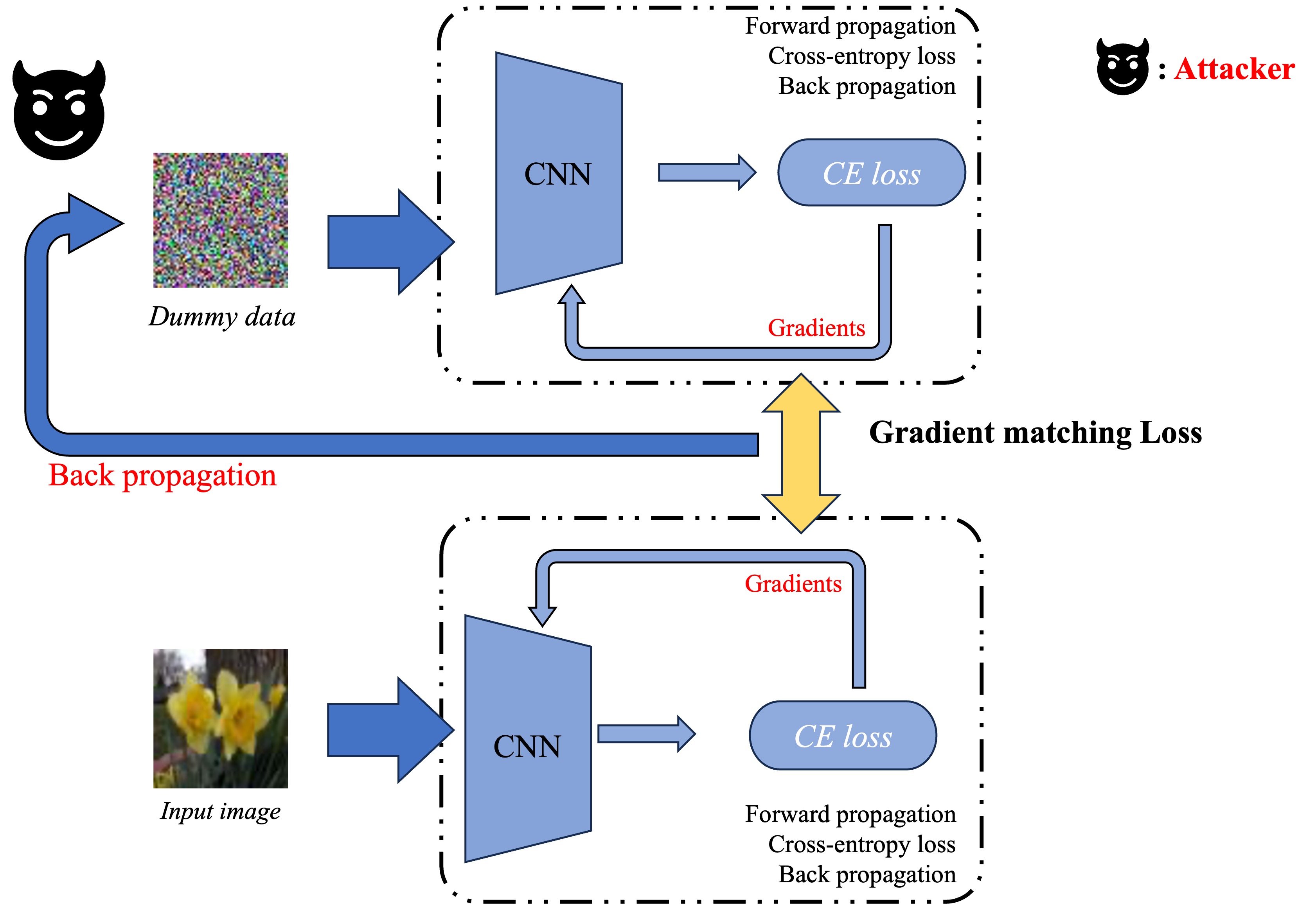
Gradient inversion attacks (GIAs) aim at reconstructing clients’ private input data from the gradients in deep neural network training phases. It is a threat to federated learning framework, especially the horizontal one where a curious-but-honest central server collects gradients from multiple clients, analyzes the optimal parameter updating direction, and sends back the updated model in one step. Getting rid of complicated mathematical formulas, GIA is actually a matching process: the attacker (which is the central server in the most common settings) expects that the data it randomly initialized could finally generate the identical gradients as the ground truth, therefore it measures the difference (or distance) to optimize input data pixel-wisely. The smaller the distance between gradients, the better the private data are reconstructed.

This is a white-box attack, for its requirement for full model parameters to conduct backpropagation. In such a process, with fixed model parameters, the distance between gradients is highly dependent on the attacker’s dummy data. GIA’s target is to optimize the distance below, where $x^\ast$ and $y^\ast$ represent the dummy data-label tuple, $\mathcal{D}$ represents the distance function, $\theta$ represents the model weights, and $\mathcal{L}$ represents the CE loss.

\[\arg\min \limits_{(x^*,y^*)} {\mathcal{D}}\left(\nabla_\theta\mathcal{L}_\theta\left( x,y\right),\nabla_\theta\mathcal{L}_\theta\left( x^*,y^*\right)\right)\]

After raising this problem, there are a few research topics in this field. iDLG provides a way to recover the input label analytically. Following this, a series of works is proposed to recover labels from batches, and it is generally believed that compared with optimizing image-label tuples simultaneously, simply optimizing input images with ground-truth labels could achieve better performance. Except for recovering labels, attack evaluations and defense methods also attract much attention. However, recovering high-quality images is still the key focus.

The tough challenge in GIAs

In GIA, the tough challenge, which has not been solved yet, is the reconstruction of batched input data, where multiple samples share the same labels. Previous works headed towards such a goal by a few steps: they first recovered single input data, then extended them to batches with known labels, and added a new algorithm to recover batched one-hot labels before recovering input images. However, to the best of my knowledge, it is still limited to the situation where for every class there could be at most one sample in a batch. Batched data recovery with repeated labels is still a failure for all current algorithms. The key reason for this failure lies in the information discard of averaged gradients.

A simple example of information discards

Let’s first take a look at a simple neural network: MLP. In a specific layer, it takes in intermediate features $\mathbf{x}$ and outputs a result of matrix multiplication $\mathbf{z}=\mathbf{Wx}+\mathbf{b}$. To recover the input from gradients, we could simply use the bias attack:

\[\frac{\partial \mathcal{L}}{\partial {\mathbf{W}}}=\frac{\partial \mathcal{L}}{\partial \mathbf{z}} \times \frac{\partial \mathbf{z}}{\partial {\mathbf{W}}}=\frac{\partial \mathcal{L}}{\partial {b}}\mathbf{x}^\mathrm{T}\]

In the above equation, it is clear that for a single input, with full access to model weights and gradients, the gradients of the MLP contain full information to execute single-image recovery.

Here, we conduct a simple experiment to illustrate the existence of information discard. Firstly We pick a 4-layer MLP as the target neural network and randomly select a few images from the Flowers-17 dataset as the private input data for recovery. We take $l_2$ loss as the gradient matching function without any prior knowledge (regularization terms). Firstly, we provide an example of input image recovery when batchsize=1 with known labels.

Image reconstruction with $l_2$ loss on MLP. no regularization terms are adopted.

It is not surprising that $l_2$ gradient matching functions could recover the input data well. Such a good performance is mainly because MLP’s gradients contain enough information of intermediate features for single inputs. With proper labels, we could conclude that GIA works well on MLP when batchsize=1.

However, when it comes to CNNs, such inversion gets harder. For convolution layers, the gradients of convolution kernels are aggregated through the whole feature map, therefore even if we set batchsize=1, gradients may still experience information discards, affecting the attack performance. This problem is also mentioned in R-GAP, which executes the GIA from an equation-solving perspective. If equations are “rank-deficient”, then we cannot get a unique solution, indicating obvious information discards. Here, for better illustration, we first show CIFAR-10 image reconstructions on LeNet with batchsize=1. Ground-truth one-hot labels are provided.

Image reconstruction on LeNet with CIFAR-10 dataset when batchsize=1. we show the ground-truth image in the middle and attach the reconstruction process on two sides ($l_2$ loss on the left and cosine similarity loss on the right).

It is clear that even though both functions could recover the image, there are some pixels not perfectly optimized, indicating the existence of information discards. If we change the batchsize, even if we only slightly enlarge it as batchsize=2, such reconstruction ends up with a failure.

Image reconstruction with cosine similarity loss on LeNet and no regularization terms are adopted. In the middle, we show ground-truth images in the batch.

For a given network, the size of gradients is fixed. Therefore, with the increase in batchsize, GIA will experience more obvious information discards. This is easy to understand, and researchers designed a few ways to complement this loss.

Understanding GIAs from the prior knowledge perspective

Realizing the information discards, reviewing the recent paper through the prior knowledge perspective may help understand the logic better. To achieve better image reconstruction quality, it is natural to consider the prior knowledge of images as the complement. Here, the prior knowledge could be explained in three aspects.

Unparameterized regularization terms

In IG, they utilize the total variance as a regularization because they believe a real image taken from nature should have a small total variance. That is the first prior knowledge term utilized in the gradient matching function, and it turns out to function well. After that, in GradInversion this regularization term is extended to include batch normalization supervision, $l_2$ norms and group consistency. This is a stronger prior knowledge implying that a real input image, or batched real images, except for total variance, should also possess lower $l_2$ norms, proper intermediate mean and the variance for batch normalization layers. Apart from that, all reconstructions from different random initializations ought to reach a group consistency. These terms are unparameterized, and it is clearly demonstrated in their ablation experiments that these terms matter significantly in reconstructing high-quality images.

To further illustrate the benefits such regulariztaion terms have on the data reconstruction processes, here is an example of adding total variance for batchsize=2 image reconstruction. The scale of total variance ranges from $10^{-4}$ to $10^{-1}$.

Image reconstruction with cosine similarity loss and total variance on LeNet. The scale of the total variance starts from $10^{-4}$ for the very left column to $10^{-1}$ with 10 times as the interval.

With identical learning rate, images with higher total variance are reconstructed faster. Because the total variance penalizes obvious distinctions for adjacent pixels, images with higher total variance are also more blurred. On the other side, reconstructions with insufficient total variance fail to generate recognizable images.

Generative models

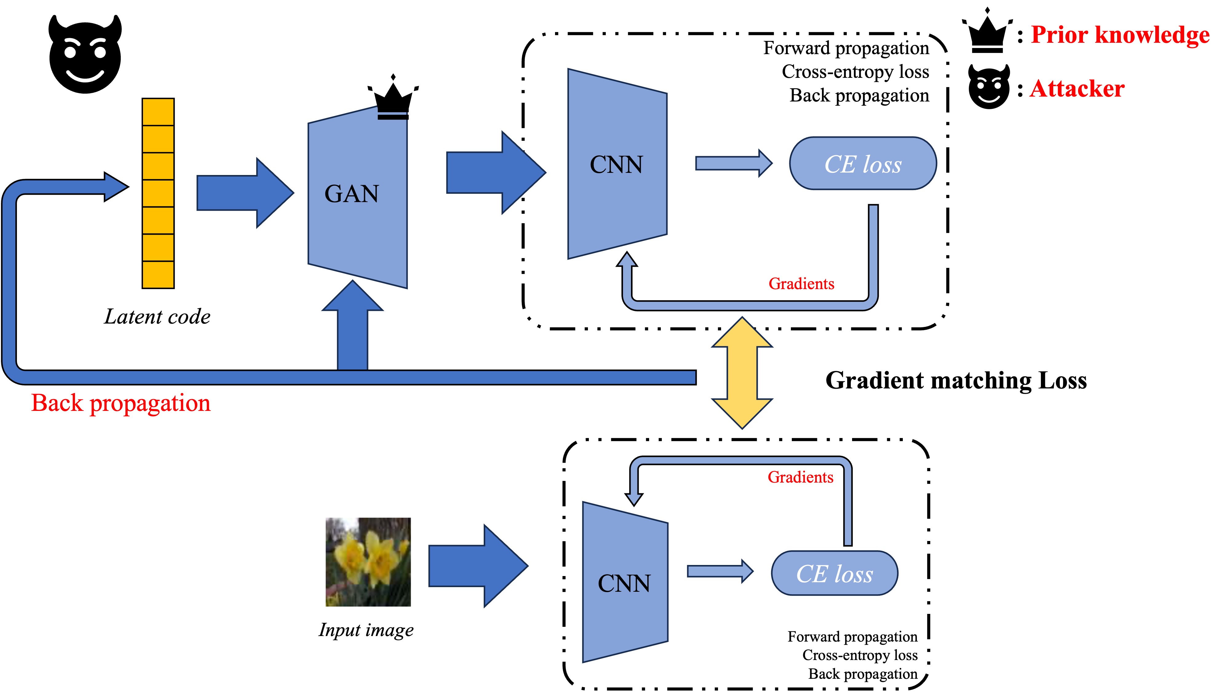
Keep following the logic that recent works require some other conditions as prior knowledge to reinforce the information discards from gradients, generative models, especially GANs, could serve as a strong tool to encode what “real images” should be. The way to add GAN’s generator in gradient matching processes is simple: instead of optimizing direct image pixels, with the generator we could keep the backpropagation way back to the latent space, then alter the latent code as well as the parameters of the generator to produce recovered images. Pre-trained generators naturally encode a likely distribution of the input data, which is a stronger prior knowledge compared with previous unparameterized regularization terms.

Recent work GIFD extends this method by optimizing GAN network layer-wisely. Instead of directly optimizing GAN weights and the latent vector in one step, GIFD optimizes the intermediate layers iteratively, making such a process more stable. In summary, gradients here serve more as an indicator for attackers to select the best image from distributions modeled by pre-trained GANs.

End-to-end networks

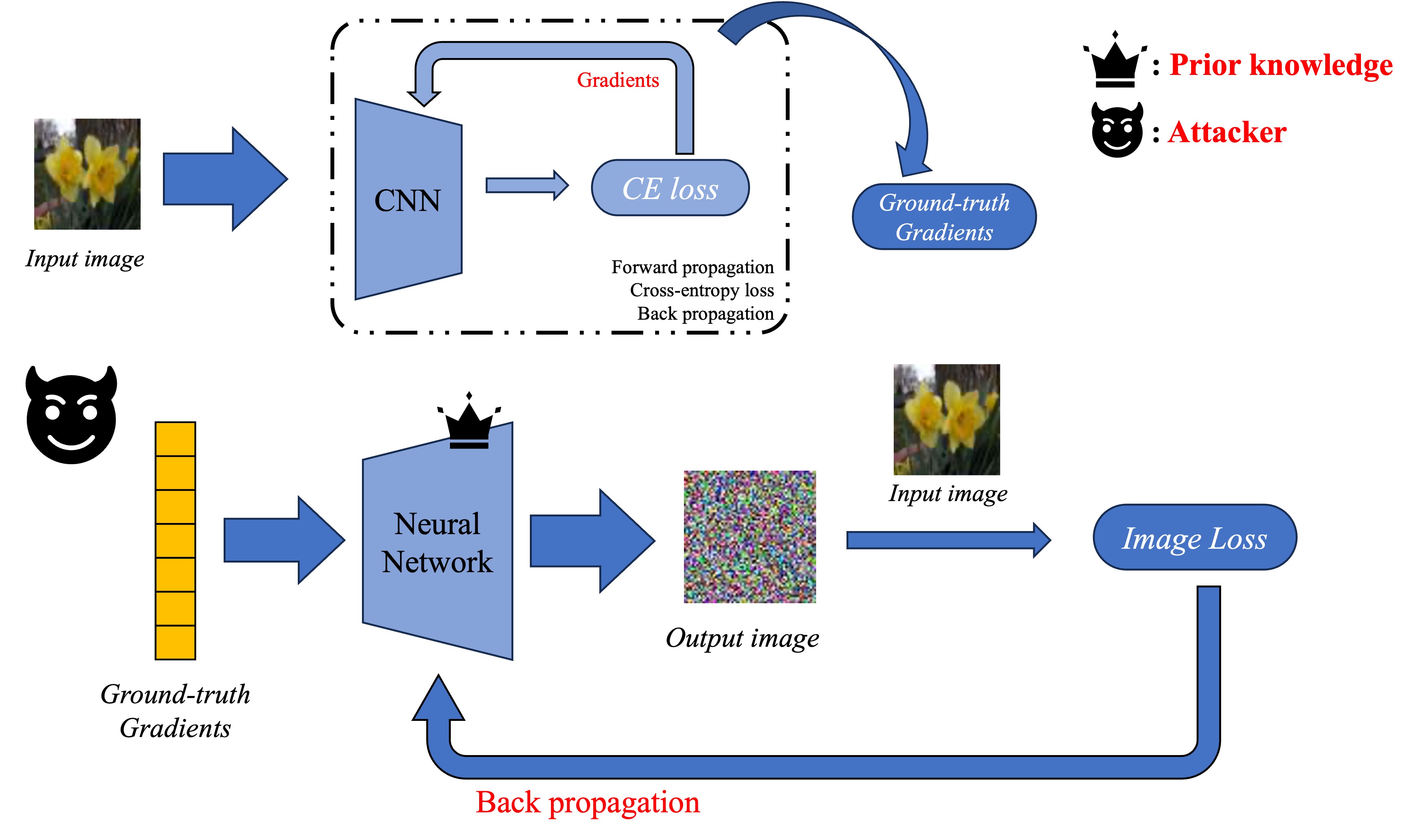
Actually, the most intuitive way to conduct a GIA is to design a function that takes gradients as input and then outputs recovered images. For a target network, image-gradient tuples are easy to collect, therefore the prior knowledge could be encoded in such an end-to-end neural network through model training.

Here, the neural network resembles a GAN generator which takes in representation vectors and outputs a synthesized image. However, instead of abstract latent codes, such a network receives gradient vectors to generate images. In implementations, Wu et.al utilizes feature hashing to reduce the dimension of gradient vectors. For network picking, they use a simple 3-layer MLP to generate flattened images, which is different from widely-used GAN structures. However, such a method faces multiple difficulties, such as large input sizes and limited structural flexibility. Even for one specific model, once the model weights are changed, such end-to-end network requires retraining to construct a new mapping from gradients to images. Besides, there is still space for network design. Will the network structure influence image reconstruction performance under identical datasets? How to construct a mapping function from gradients to images with varying batchsize? Could the network find an optimal batchsize after analyzing the gradients? These questions are all worth further exploration.

Limitation and future directions

For GIAs that require pre-trained models, the key limitation is the auxiliary dataset. It is kind of unrealistic to claim that the dataset used for pretraining generative models (or end-to-end models) shares the same distribution with the unknown private input data, and possibly, with distinct dataset distribution, the generative performance may experience a drop. Both GIAS and GIFD use GAN with in-distribution auxiliary data to compare with previous state-of-the-art works, and GIFD paper only shows the reconstruction result of distinct distribution data when batchsize=1 with the same label space. For the most general situation where the attacker has limited knowledge of the potential distribution of the private data, it may be still hard to recover high-quality batched data with generative networks. Considering these limitations, it is of great value to explore algorithms to learn some general prior knowledge, especially those robust among different data distributions.

Conclusions

The existence of information discards in gradient aggregation is the tough challenge of GIAs.
From the prior knowledge perspective, previous GIA works provide three ways to complement information discards.
It may still be hard to recover batched data from gradients with limited knowledge of private data distribution.