Towards Robust Foundation Models: Adversarial Contrastive Learning
Foundation models pre-trained on large-scale unlabelled datasets using self-supervision can be generalizable to a wide range of downstream tasks. Existing work has shown that adversarial attacks can effectively fool any downstream models fine-tuned from a pre-trained foundation model. The existence of such adversarial attacks necessitates the development of robust foundation models which can yield both standard generalization and adversarial robustness to safety-critical downstream tasks. Currently, adversarial contrastive learning (ACL) is one of the most effective methods for outputting a robust foundation model. ACL incorporates contrastive learning with adversarial data to effectively output a robust representation without requiring costly annotations. In this blog, we introduced two NeurIPS 2023 publications that can enhance ACL's efficacy and efficiency, respectively. (1) This blog introduces Adversarial Invariant Regularization (AIR) which is a state-of-the-art ACL algorithm. A causal theoretical framework is built to interpret ACL, and then the AIR algorithm is derived from the causal framework to regulate and improve the ACL. (2) This blog also introduces a Robustness-aware Coreset Selection (RCS) method to speed up ACL. RCS does not require label information and searches for an informative training subset that can maintain the adversarial robustness. For the first time, RCS enables the application of ACL on the large-scale ImageNet-1K dataset.
Foundation Models
Foundation models

Contrastive Learning (CL)
To build foundation models, contrastive learning (CL)
Let \(f_\theta: \mathcal{X} \rightarrow \mathcal{Z}\) be a feature extractor parameterized by \(\theta\), \(g:\mathcal{Z} \rightarrow \mathcal{V}\) be a projection head that maps representations to the space where the contrastive loss is applied, and \(\tau_i, \tau_j: \mathcal{X} \rightarrow \mathcal{X}\) be two transformation operations randomly sampled from a pre-defined transformation set \(\mathcal{T}\). Given a mini-batch \(B \sim \mathcal{X}^\beta\) consisting of \(\beta\) samples, we denote the augmented minibatch \(B^\prime = \{ \tau_i(x_k), \tau_j(x_k) \mid \forall x_k \in B \}\) consisting of \(2\beta\) samples. We take \(h_\theta(\cdot) = g \circ f_\theta(\cdot)\) and \(x_k^u = \tau_u(x_k)\) for any \(x_k \sim \mathcal{X}\) and \(u \in \{i,j\}\). The contrastive loss between different natural views (i.e., \(x_k^i\) and \(x_k^j\)) is formulated as follows:
\[\ell_\mathrm{CL}(x_k^i,x_k^j; \theta)\!=\!-\! \sum\limits_{u \in \{i,j\}} \! \log \frac{e^{\mathrm{sim} \left(h_\theta(x_k^i), h_\theta(x_k^j) \right)/t}}{\sum\limits_{x \in B^\prime \setminus \{x_k^u\}} e^{\mathrm{sim} \left( h_\theta(x_k^u), h_\theta(x) \right)/t}},\]where \(\mathrm{sim}(\cdot,\cdot)\) is the cosine similarity function.

How to implement CL at the pre-training stage in practice?
Click here to see the Pytorch code for calculating contrastive loss. You can copy-paste it to calculate the contrastive loss in convenience. The code is copied from https://github.com/GodXuxilie/Enhancing_ACL_via_AIR.
import torch
import torch.nn as nn
import torch.nn.functional as F

class CL(nn.Module):

    def __init__(self, normalize=True, temperature=0.5):
        super(CL, self).__init__()
        self.normalize = normalize
        self.temperature = temperature

    def forward(self, zi, zj):
        # zi: the representation of natural view x^i.
        # zj: the representation of natural view x^j.

        bs = zi.shape[0]
        labels = torch.zeros((2*bs,)).long().to(zi.device)
        mask = torch.ones((bs, bs), dtype=bool).fill_diagonal_(0)

        zi_norm = F.normalize(zi, p=2, dim=-1) if self.normalize else zi
        zj_norm = F.normalize(zj, p=2, dim=-1) if self.normalize else zj

        ### Contrastive Loss ###
        logits_ii = torch.mm(zi_norm, zi_norm.t()) / self.temperature
        logits_ij = torch.mm(zi_norm, zj_norm.t()) / self.temperature
        logits_ji = torch.mm(zj_norm, zi_norm.t()) / self.temperature
        logits_jj = torch.mm(zj_norm, zj_norm.t()) / self.temperature

        logits_ij_pos = logits_ij[torch.logical_not(mask)]
        logits_ji_pos = logits_ji[torch.logical_not(mask)]
        logits_ii_neg = logits_ii[mask].reshape(bs, -1)
        logits_ij_neg = logits_ij[mask].reshape(bs, -1)
        logits_ji_neg = logits_ji[mask].reshape(bs, -1)
        logits_jj_neg = logits_jj[mask].reshape(bs, -1)

        pos = torch.cat((logits_ij_pos, logits_ji_pos), dim=0).unsqueeze(1)
        neg_i = torch.cat((logits_ii_neg, logits_ij_neg), dim=1)
        neg_j = torch.cat((logits_ji_neg, logits_jj_neg), dim=1)
        neg = torch.cat((neg_i, neg_j), dim=0)

        logits = torch.cat((pos, neg), dim=1)
        nat_contrastive_loss = F.cross_entropy(logits, labels)
        return nat_contrastive_loss
Besides, you can use the following script to conduct self-supervised pre-training via CL using ResNet-18 on CIFAR-10:
# Pre-training stage via CL
git clone https://github.com/GodXuxilie/Enhancing_ACL_via_AIR.git
cd Enhancing_ACL_via_AIR
PRE_TRAIN_DIR=CL_ResNet18_cifar10
python pretraining.py $PRE_TRAIN_DIR --dataset cifar10 \
                                     --model r18 \
                                     --pgd_iter 0  --lambda1 0 --lambda2 0
Robust Foundation Models
Existing work

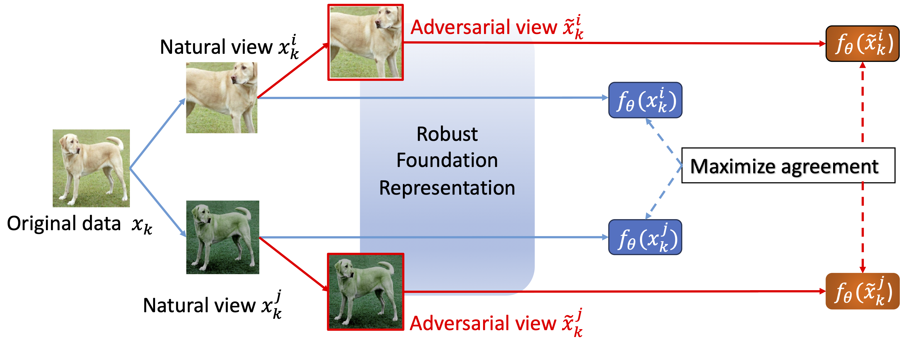
Robust foundation models are pre-trained on large-scale datasets via robust self-supervised learning methods. Robust foundation models have the following two critical properties:
- Robust foundation representations is generalizable to downstream tasks;
- Fine-tuned robust foundation representations is adversarially robust against adversarial attacks in downstream tasks.

Adversarial Contrastive Learning (ACL)
To learn robust foundation representations, adversarial contrastive learning (ACL)
where adversarial views are formulated as follows:
\[\tilde{x}_{k}^i, \tilde{x}_{k}^j = \mathop{\arg\max}_{ {\Large \tilde{x}_{k}^i \in \mathcal{B}_\epsilon[x_k^i]} \atop {\Large \tilde{x}_{k}^j \in \mathcal{B}_\epsilon[x_k^j]} } \ell_\mathrm{CL}(\tilde{x}_{k}^i, \tilde{x}_{k}^j; \theta).\]Note that \(\omega \in [0,1]\) is a scalar and \(\mathcal{B}_\epsilon[x]\) is a constraint that ensures the adversarial data \(\tilde{x}\) is in the \(\epsilon\)-ball around data \(x\).
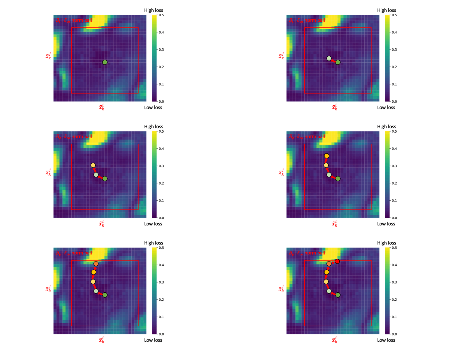
Here is the generation procedure of adversarial data via Projected Gradient Descent (PGD)
where \(\Pi_{\mathcal{B}_\epsilon[x]}\) projects the data into the \(\epsilon\)-ball around the initial point \(x\). Generating adversarial data requires \(T\) iterations of forwarding and back-propagations, which makes the training procedure extremely slow.
At each epoch, ACL conducts steps (1) and (2) alternatively:
-
Step (1): generating adversarial data (i.e., \(\tilde{x}_k^i\) and \(\tilde{x}_k^j\)) via PGD;
-
Step (2): updating model parameters via minimizing adversarial contrastive loss to maximize agreements on the adversarial data and natural data.
How to implement ACL at the pre-training stage in practice?
Click here to see the Pytorch code for calculating adversarial contrastive loss. You can copy-paste it to calculate the adversarial contrastive loss in convenience. The code is copied from https://github.com/GodXuxilie/Enhancing_ACL_via_AIR.
import torch
import torch.nn as nn
import torch.nn.functional as F

class ACL(nn.Module):

    def __init__(self, normalize=True, temperature=0.5):
        super(ACL, self).__init__()
        self.normalize = normalize
        self.temperature = temperature

    def forward(self, zi, zj, zi_adv, zj_adv, weight=0.5):
        # zi: the representation of natural view x^i.
        # zj: the representation of natural view x^j.
        # zi_adv: the representation of adversarial view \tilde{x}^i.
        # zj_adv: the representation of adversarial view \tilde{x}^j.

        bs = zi.shape[0]
        labels = torch.zeros((2*bs,)).long().to(zi.device)
        mask = torch.ones((bs, bs), dtype=bool).fill_diagonal_(0)

        zi_norm = F.normalize(zi, p=2, dim=-1) if self.normalize else zi
        zj_norm = F.normalize(zj, p=2, dim=-1) if self.normalize else zj
        zi_adv_norm = F.normalize(zi_adv, p=2, dim=-1) if self.normalize else zi_adv
        zj_adv_norm = F.normalize(zj_adv, p=2, dim=-1) i if self.normalize else zj_adv

        ### Adversarial Contrastive Loss ###

        logits_ii = torch.mm(zi_norm, zi_norm.t()) / self.temperature
        logits_ij = torch.mm(zi_norm, zj_norm.t()) / self.temperature
        logits_ji = torch.mm(zj_norm, zi_norm.t()) / self.temperature
        logits_jj = torch.mm(zj_norm, zj_norm.t()) / self.temperature

        logits_ij_pos = logits_ij[torch.logical_not(mask)]
        logits_ji_pos = logits_ji[torch.logical_not(mask)]
        logits_ii_neg = logits_ii[mask].reshape(bs, -1)
        logits_ij_neg = logits_ij[mask].reshape(bs, -1)
        logits_ji_neg = logits_ji[mask].reshape(bs, -1)
        logits_jj_neg = logits_jj[mask].reshape(bs, -1)

        pos = torch.cat((logits_ij_pos, logits_ji_pos), dim=0).unsqueeze(1)
        neg_i = torch.cat((logits_ii_neg, logits_ij_neg), dim=1)
        neg_j = torch.cat((logits_ji_neg, logits_jj_neg), dim=1)
        neg = torch.cat((neg_i, neg_j), dim=0)

        logits = torch.cat((pos, neg), dim=1)
        nat_contrastive_loss = F.cross_entropy(logits, labels)

        logits_ii_adv = torch.mm(zi_adv_norm, zi_adv_norm.t()) / self.temperature
        logits_ij_adv = torch.mm(zi_adv_norm, zj_adv_norm.t()) / self.temperature
        logits_ji_adv = torch.mm(zj_adv_norm, zi_adv_norm.t()) / self.temperature
        logits_jj_adv = torch.mm(zj_adv_norm, zj_adv_norm.t()) / self.temperature

        logits_ij_pos_adv = logits_ij_adv[torch.logical_not(mask)]
        logits_ji_pos_adv = logits_ji_adv[torch.logical_not(mask)]
        logits_ii_neg_adv = logits_ii_adv[mask].reshape(bs, -1)
        logits_ij_neg_adv = logits_ij_adv[mask].reshape(bs, -1)
        logits_ji_neg_adv = logits_ji_adv[mask].reshape(bs, -1)
        logits_jj_neg_adv = logits_jj_adv[mask].reshape(bs, -1)

        pos_adv = torch.cat((logits_ij_pos_adv, logits_ji_pos_adv), dim=0).unsqueeze(1)
        neg_i_adv = torch.cat((logits_ii_neg_adv, logits_ij_neg_adv), dim=1)
        neg_j_adv = torch.cat((logits_ji_neg_adv, logits_jj_neg_adv), dim=1)
        neg_adv = torch.cat((neg_i_adv, neg_j_adv), dim=0)

        logits_adv = torch.cat((pos_adv, neg_adv), dim=1)
        adv_contrastive_loss = F.cross_entropy(logits_adv, labels)

        return (1 - weight) * nat_contrastive_loss + (1 + weight) * adv_contrastive_loss
Besides, you can use the following script to conduct robust self-supervised pre-training via ACL using ResNet-18 on CIFAR-10:
# Pre-training stage via ACL
git clone https://github.com/GodXuxilie/Enhancing_ACL_via_AIR.git
cd Enhancing_ACL_via_AIR
PRE_TRAIN_DIR=ACL_ResNet18_cifar10
python pretraining.py $PRE_TRAIN_DIR --dataset cifar10 \
                                     --model r18 \
                                     --DynAug --lambda1 0 --lambda2 0
How to utilize robust foundation representations via fine-tuning in downstream tasks?
At the fine-tuning stage, a classifier is randomly initialized and appended to the pre-trained feature extractor for solving the classification tasks. There are three types of fine-tuning modes:
- Standard linear fine-tuning (SLF): only standardly fine-tuning the classifier while freezing the feature extractor.
- Adversarial linear fine-tuning (ALF): only adversarially fine-tuning the classifier while freezing the feature extractor.
- Adversarial full fine-tuning (AFF): adversarially fine-tuning both the feature extractor and the classifier.
You can use the following script to transfer an adversarially pre-trained ResNet-18 on CIFAR-10 to a downstream task CIFAR-100 via fine-tuning:
# Fine-tuning stage
cd Enhancing_ACL_via_AIR
PRE_TRAIN_DIR=ACL_ResNet18_cifar10
FINETUNE_DIR=ACL_ResNet18_cifar10_cifar100
MODE=SLF/ALF/AFF/ALL
python finetuning.py --mode $MODE \
                     --experiment $FINETUNE_DIR \
                     --checkpoint ./checkpoints/$PRE_TRAIN_DIR/model.pt \
                     --dataset cifar100 \
                     --model r18 \
                     --eval-AA --eval-OOD --pretraining DynACL
Note that MODE=ALL refers to that the finetuning.py sequentially conducts fine-tuning of all three modes (i.e., SLF, ALF, and AFF) and outputs the result via each fine-tuning mode in the log file $FINETUNE_DIR/results/log.txt.
Enhancing ACL via Adversarial Invariant Regularization (AIR)
Here, we introduce the NeurIPS 2023 paper
Causal View of ACL
AIR
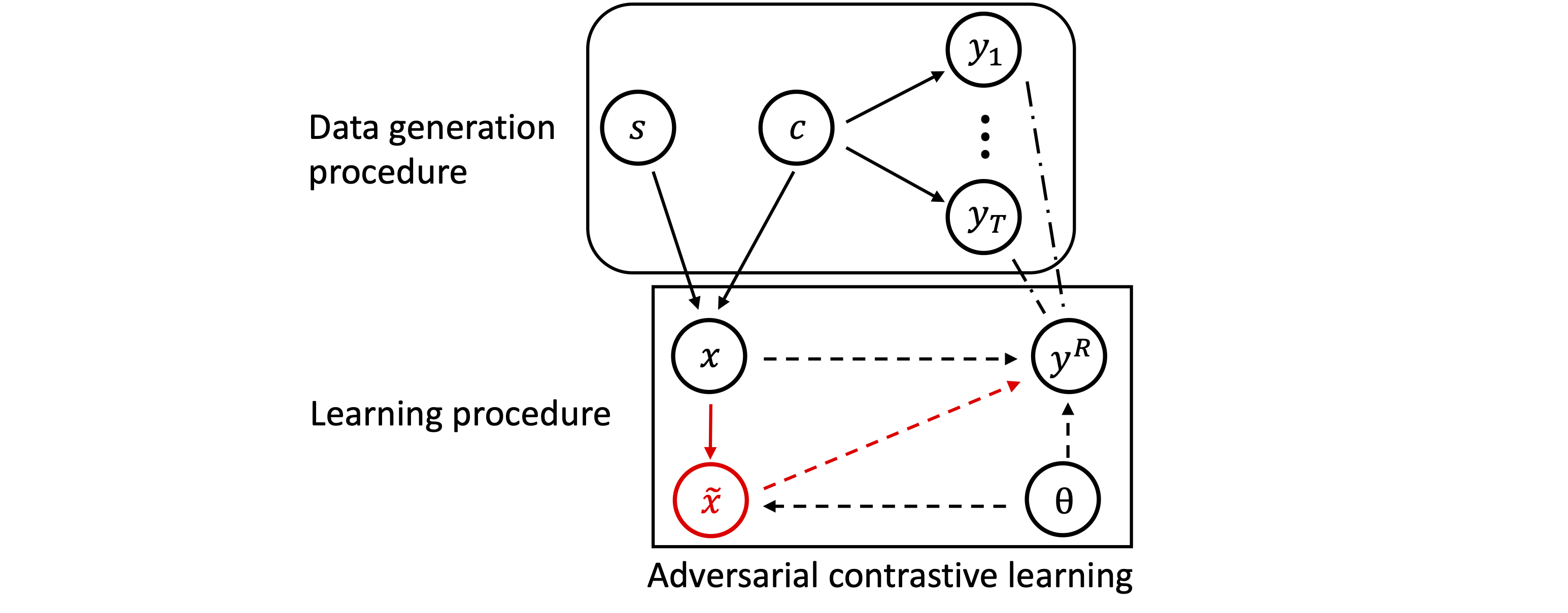
During the data generation procedure:
- \(c\) is the content variable, which can be regarded as the original data in the datasets.
- \(s\) is the style factor, which can regarded as the data transformation functions that can modify the content while maintaining the semantic meaning of the content. Note that factors \(c\) and \(s\) are independent.
- \(x\) is the natural data, which is decided by the content factor \(c\) and the style factor \(s\).
- \(y_t \in \{ y_i \}_{i=1}^{T}\) is the label from an unknown downstream task. Note that \(y_t\) is only decided by the content factor \(c\).
- \(y^R\) is the proxy label, which is a refinement of $y_t$. \(y^R\) is used for self-supervised learning without labels. As illustrated in the following figure, the label
dogis refined into proxy labelsgolden Retriever with yellow hairandlabrador retriever with black hair. Therefore, when there is no target label, we can train models by differentiating these two different pictures using the contrastive loss.

- \(\tilde{x}\) is the adversarial data of $x$. Since the generation procedure of \(\tilde{x}\) in ACL does not use the labels, the adversarial data \(\tilde{x}\) is decided by the natural data \(x\) and the model parameter \(\theta\).
During the learning procedure, ACL optimizes the parameters \(\theta\) by maximizing the conditional probabilities both \(p(y^R \mid x)\) and \(p(y^R \mid \tilde{x})\).
the Methodology of AIR
Style-invariant criterion.
From the causal view of ACL, the learning procedure should satisfy the style-independent criterion. That is to say, the intervention on the style factor should not affect the conditional probability, i.e., \(p^{do(\tau_i)}(y^R \mid x) = p^{do(\tau_j)}(y^R \mid x)\) where \(do(\tau)\) is the intervention approximated by the data augmentation function $\tau \in \mathcal{T}$.
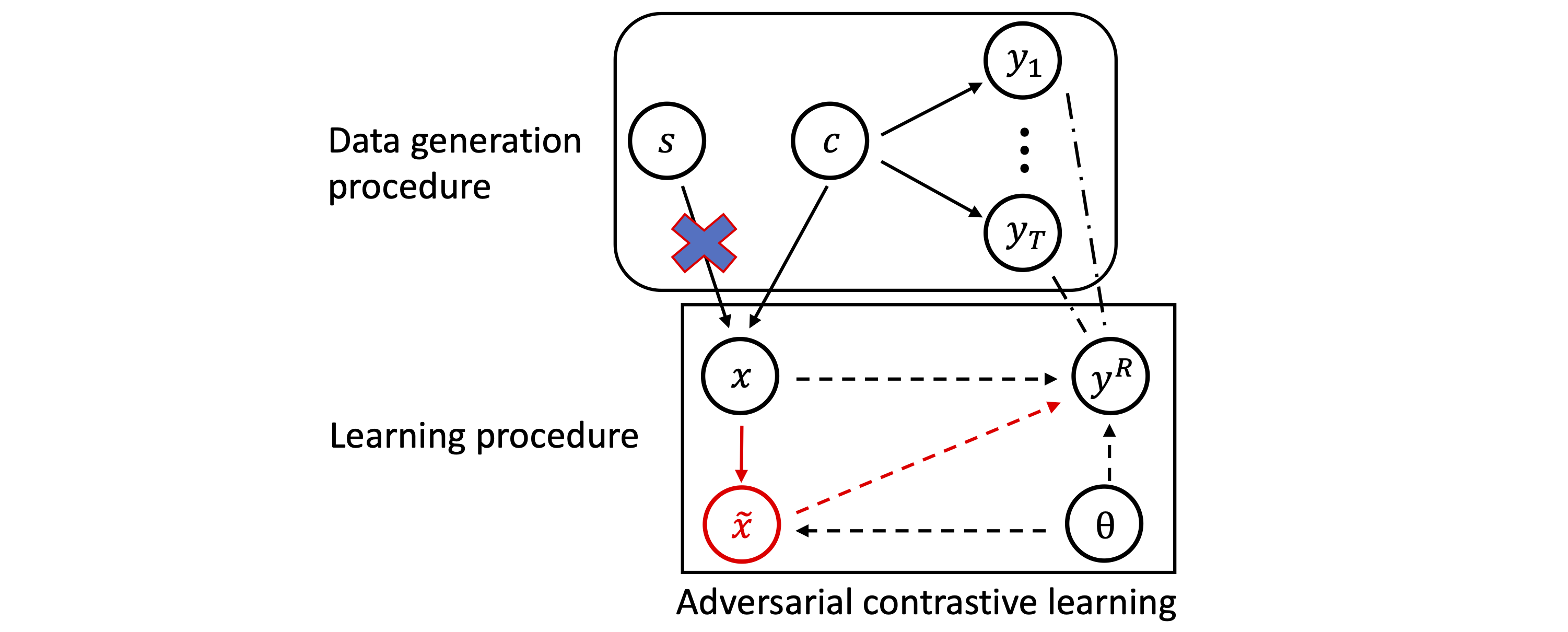
Assuming that the path \(x \rightarrow \tilde{x} \rightarrow y^R\) in the causal graph satisfies the Markov condition, we can obtain that
\[p(y^R \mid x) = p(y^R \mid \tilde{x})p(\tilde{x} \mid x).\]Therefore, ACL should follow the style-independent criterion as follows:
\[p^{do(\tau_i)}(y^R \mid \tilde{x}) p^{do(\tau_i)}(\tilde{x} \mid x) = p^{do(\tau_j)}(y^R \mid \tilde{x}) p^{do(\tau_j)}(\tilde{x} \mid x) \quad \forall \tau_i, \tau_j \in \mathcal{T} .\]The conditional probability \(p^{do(\tau_u)}(y^R \mid \tilde{x})\) for \(u \in \{i,j\}\) is calculated as the cosine similarity between the original data \(x\) and the adversarial data \(\tilde{x}^u\) normalized by the softmax function:
\[p^{do(\tau_u)}(y^R \mid \tilde{x}) = \frac{e^{\mathrm{sim} \left(f_\theta(x), f_\theta(\tilde{x}^u) \right)/t}} {\sum\limits_{x_k \in B} e^{\mathrm{sim} \left( f_\theta(x_k), f_\theta(\tilde{x}_k^u) \right)/t}}.\]Note that \(y^R\) is only decided by the content factor \(c\). Empirically, the content factor \(c\) can be approximated by the original data \(x\) from the datasets.
The conditional probability \(p^{do(\tau_u)}(\tilde{x} \mid x)\) for \(u \in \{i,j\}\) is calculated as the cosine similarity between the natural data \(x^u\) and the adversarial data \(\tilde{x}^u\) normalized by the softmax function:
\[p^{do(\tau_u)}(\tilde{x} | x) = \frac{e^{\mathrm{sim} \left(f_\theta(\tilde{x}^u), f_\theta(x^u) \right)/t}} {\sum\limits_{x_k \in B} e^{\mathrm{sim} \left( f_\theta(\tilde{x}_k^u), f_\theta(x_k^u) \right)/t}}.\]The loss function of AIR.
To achieve the style-invariant criterion, AIR is proposed to regulate the representations to be style-independent as follows:
\[\mathcal{L}_\mathrm{AIR}(B;\theta, \epsilon) = \mathrm{KL}\left(p^{do(\tau_i)}(y^R \mid \tilde{x}) p^{do(\tau_i)}(\tilde{x} \mid x) \| p^{do(\tau_j)}(y^R \mid \tilde{x}) p^{do(\tau_j)}(\tilde{x} \mid x) ; B \right),\]in which \(\epsilon \geq 0\) is the adversarial budget, \(B\) is a mini-batch, and \(\mathrm{KL}(p(x) \| q(x); B) = \sum_{x \in B} p(x) \log \frac{p(x)}{q(x)}\) denotes the Kullback–Leibler (KL) divergence.
We provide an illustration of AIR for ACL. The AIR aims to maximize the agreements between the original data and the adversarial view (the dash yellow lines) and the agreements between the natural view and the adversarial view (the dash pink lines).
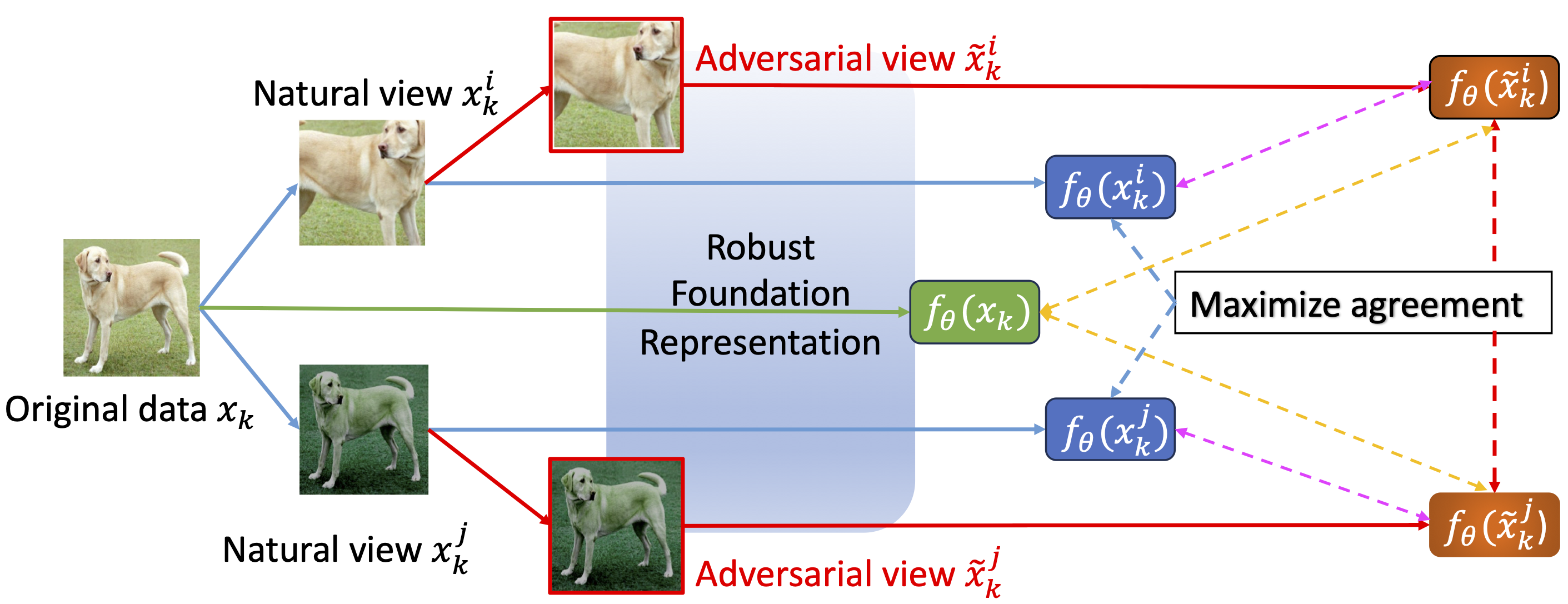
Learning objective of AIR enhanced ACL.
The learning objective of AIR is formulated as follows:
\[\mathop{\arg\min}_{\theta} \sum_{x \in U} \ell_\mathrm{ACL}(x; \theta) + \lambda_1 \cdot \mathcal{L}_\mathrm{AIR}(U;\theta,0) + \lambda_2 \cdot \mathcal{L}_\mathrm{AIR}(U;\theta,\epsilon),\]where \(\lambda_1 \geq 0\) and \(\lambda_2 \geq 0\) are two hyper-parameters.
The official code of AIR is available at https://github.com/GodXuxilie/Enhancing_ACL_via_AIR.
Click here to see the Pytorch code for calculating AIR loss. You can copy-paste it to calculate the AIR loss in convenience.
import torch
import torch.nn as nn
import torch.nn.functional as F

class AIR(nn.Module):

    def __init__(self, normalize=True, temperature=0.5):
        super(AIR, self).__init__()
        self.normalize = normalize
        self.temperature = temperature

    def forward(self, zi, zj, zi_adv, zj_adv, z_orig, weight=0.5, lambda1=0.5, lambda2=0.5):
        # zi: the representation of natural data x^i.
        # zj: the representation of natural data x^j.
        # zi_adv: the representation of adversarial data \tilde{x}^i.
        # zj_adv: the representation of adversarial data \tilde{x}^j.
        # z_orig: the representation of original data x.

        bs = zi.shape[0]
        labels = torch.zeros((2*bs,)).long().to(zi.device)
        mask = torch.ones((bs, bs), dtype=bool).fill_diagonal_(0)

        zi_norm = F.normalize(zi, p=2, dim=-1) if self.normalize else zi
        zj_norm = F.normalize(zj, p=2, dim=-1) if self.normalize else zj
        zi_adv_norm = F.normalize(zi_adv, p=2, dim=-1) if self.normalize else zi_adv
        zj_adv_norm = F.normalize(zj_adv, p=2, dim=-1) if self.normalize else zj_adv
        zo_norm = F.normalize(z_orig, p=2, dim=-1) if self.normalize else z_orig

        ### Adversarial Contrastive Loss ###
        logits_ii = torch.mm(zi_norm, zi_norm.t()) / self.temperature
        logits_ij = torch.mm(zi_norm, zj_norm.t()) / self.temperature
        logits_ji = torch.mm(zj_norm, zi_norm.t()) / self.temperature
        logits_jj = torch.mm(zj_norm, zj_norm.t()) / self.temperature

        logits_ij_pos = logits_ij[torch.logical_not(mask)]
        logits_ji_pos = logits_ji[torch.logical_not(mask)]
        logits_ii_neg = logits_ii[mask].reshape(bs, -1)
        logits_ij_neg = logits_ij[mask].reshape(bs, -1)
        logits_ji_neg = logits_ji[mask].reshape(bs, -1)
        logits_jj_neg = logits_jj[mask].reshape(bs, -1)

        pos = torch.cat((logits_ij_pos, logits_ji_pos), dim=0).unsqueeze(1)
        neg_i = torch.cat((logits_ii_neg, logits_ij_neg), dim=1)
        neg_j = torch.cat((logits_ji_neg, logits_jj_neg), dim=1)
        neg = torch.cat((neg_i, neg_j), dim=0)

        logits = torch.cat((pos, neg), dim=1)
        nat_contrastive_loss = F.cross_entropy(logits, labels)

        logits_ii_adv = torch.mm(zi_adv_norm, zi_adv_norm.t()) / self.temperature
        logits_ij_adv = torch.mm(zi_adv_norm, zj_adv_norm.t()) / self.temperature
        logits_ji_adv = torch.mm(zj_adv_norm, zi_adv_norm.t()) / self.temperature
        logits_jj_adv = torch.mm(zj_adv_norm, zj_adv_norm.t()) / self.temperature

        logits_ij_pos_adv = logits_ij_adv[torch.logical_not(mask)]
        logits_ji_pos_adv = logits_ji_adv[torch.logical_not(mask)]
        logits_ii_neg_adv = logits_ii_adv[mask].reshape(bs, -1)
        logits_ij_neg_adv = logits_ij_adv[mask].reshape(bs, -1)
        logits_ji_neg_adv = logits_ji_adv[mask].reshape(bs, -1)
        logits_jj_neg_adv = logits_jj_adv[mask].reshape(bs, -1)

        pos_adv = torch.cat((logits_ij_pos_adv, logits_ji_pos_adv), dim=0).unsqueeze(1)
        neg_i_adv = torch.cat((logits_ii_neg_adv, logits_ij_neg_adv), dim=1)
        neg_j_adv = torch.cat((logits_ji_neg_adv, logits_jj_neg_adv), dim=1)
        neg_adv = torch.cat((neg_i_adv, neg_j_adv), dim=0)

        logits_adv = torch.cat((pos_adv, neg_adv), dim=1)
        adv_contrastive_loss = F.cross_entropy(logits_adv, labels)

        ### Adversarial Invariant Regularization ###
        logits_io = torch.mm(zi_norm, zo_norm.t()) / self.temperature
        logits_jo = torch.mm(zj_norm, zo_norm.t()) / self.temperature
        probs_io_zi = F.softmax(logits_io[torch.logical_not(mask)], -1)
        probs_jo_zj = F.log_softmax(logits_jo[torch.logical_not(mask)], -1)
        AIR_standard = F.kl_div(probs_io_zi, probs_jo_zj, log_target=True, reduction="sum")

        logits_io = torch.mm(zi_adv_norm, zi_norm.t()) / self.temperature
        logits_jo = torch.mm(zj_adv_norm, zj_norm.t()) / self.temperature
        probs_io_zi_adv_consis = F.softmax(logits_io[torch.logical_not(mask)], -1)
        probs_jo_zj_adv_consis = F.softmax(logits_jo[torch.logical_not(mask)], -1)

        logits_io = torch.mm(zi_adv_norm, zo_norm.t()) / self.temperature
        logits_jo = torch.mm(zj_adv_norm, zo_norm.t()) / self.temperature
        probs_io_zi_adv = F.softmax(logits_io[torch.logical_not(mask)], -1)
        probs_jo_zj_adv = F.softmax(logits_jo[torch.logical_not(mask)], -1)

        probs_io_zi_adv = torch.mul(probs_io_zi_adv, probs_io_zi_adv_consis)
        probs_jo_zj_adv = torch.mul(probs_jo_zj_adv, probs_jo_zj_adv_consis)
        AIR_robust = F.kl_div(probs_io_zi_adv, torch.log(probs_jo_zj_adv), log_target=True, reduction="sum")

        return (1 - weight) * nat_contrastive_loss + (1 + weight) * adv_contrastive_loss + lambda1 * AIR_standard + lambda2 * AIR_robust
Besides, you can use the following script to conduct robust self-supervised pre-training via AIR using ResNet-18 on CIFAR-10:
# Pre-training stage via AIR
git clone https://github.com/GodXuxilie/Enhancing_ACL_via_AIR.git
cd Enhancing_ACL_via_AIR
PRE_TRAIN_DIR=AIR_ResNet18_cifar10
python pretraining.py $PRE_TRAIN_DIR --dataset cifar10 --model r18 --DynAug
Empirical Results
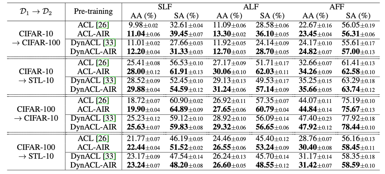
AIR yields state-of-the-art cross-task robustness transferability against adversarial attacks.
- \(\mathcal{D}_1 \rightarrow \mathcal{D}_2\) refers to that the model is pre-trained on dataset \(\mathcal{D}_1\) and fine-tuned on downstream dataset \(\mathcal{D}_2\).
-
SArefers the standard accuracy calculated as the average accuracy on the natural test data in the downstream dataset \(\mathcal{D}_2\). -
AArefers to the robust accuracy calculated as the average accuracy on the adversarial test data generated via adversarial attacks in the downstream dataset \(\mathcal{D}_2\).
AIR yields state-of-the-art cross-task robustness transferability against common corruptions.
CS-# refers to the the average accuracy evaluated on the test data under common corruptions with corruption severity (CS) of # \(\in\) {1,3,5} in the downstream dataset \(\mathcal{D}_2\).

To reproduce the above results of the transferability from CIFAR-10 to CIFAR-100, you can use the following scripts.
- At the pre-training stage, you can conduct AIR using ResNet-18 on CIFAR-10.
# Pre-training stage using AIR
git clone https://github.com/GodXuxilie/Enhancing_ACL_via_AIR.git
cd Enhancing_ACL_via_AIR
PRE_TRAIN_DIR=AIR_ResNet18_cifar10
python pretraining.py $PRETRAIN_DIR --dataset cifar10 --model r18 --DynAug- At the fine-tuning stage, you can fine-tune the pre-trained ResNet-18 to downstream task CIFAR-100. During the fine-tuning stage, the following script will automatically conduct all three fine-tuning modes (i.e., SLF, ALF, and AFF). After the fine-tuning stage, you can check the standard accuracy, the robust accuracy under adversarial attacks and common cottuptions under each fine-tuning method from a log file at
$FINETUNE_DIR/results/log.txt.
# Fine-tuning stage
cd Enhancing_ACL_via_AIR
PRE_TRAIN_DIR=AIR_ResNet18_cifar10
FINETUNE_DIR=AIR_ResNet18_cifar10_cifar100
python finetuning.py --experiment $EXP_DIR \
                     --checkpoint ./checkpoints/$PRE_TRAIN_DIR/model.pt \
                     --dataset cifar100 \
                     --model r18 \
                     --mode ALL \
                     --eval-AA --eval-OOD --pretraining DynACL_AIR
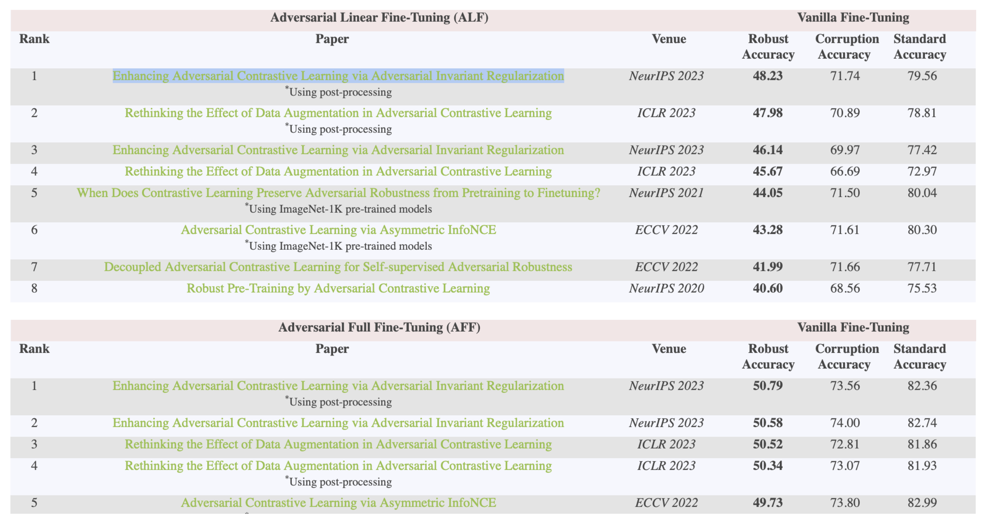
Robust Self-Supervised Learning (RobustSSL) Benchmark The website of RobustSSL Benchmark is at https://robustssl.github.io/.
AIR ranks FIRST in RobustSSL Benchmark! For more information regarding the leaderboards, please check the website of RobustSSL Benchmark.
Efficient ACL via Robustness-Aware Coreset Selection (RCS)
Here, we introduce the NeurIPS 2023 spotlight paper
Motivation—ACL is Inefficient
ACL is computationally prohibitive on large-scale datasets since generating adversarial data requires expensive computational overheads.
Empirically, ACL on the entire ImageNet-1K dataset (1,281,167 training data points) requires about 650 hours evaluated on RTX A5000 GPUs. Due to the inefficiency of ACL, ACL has not yet been applied to ImageNet-1K datasets without RCS.

the Methodology of RCS
Intuition of RCS.
To speed up ACL, RCS takes an intuitive idea which is to find an informative training subset (called “coreset”). The coreset can directly decrease the number of training samples, thus significantly accelerating ACL. Besides, since the coreset is informative, which is beneficial in improving \(f\)’s adversarial robustness, it should guarantee the ACL to output an effective robust foundation model.
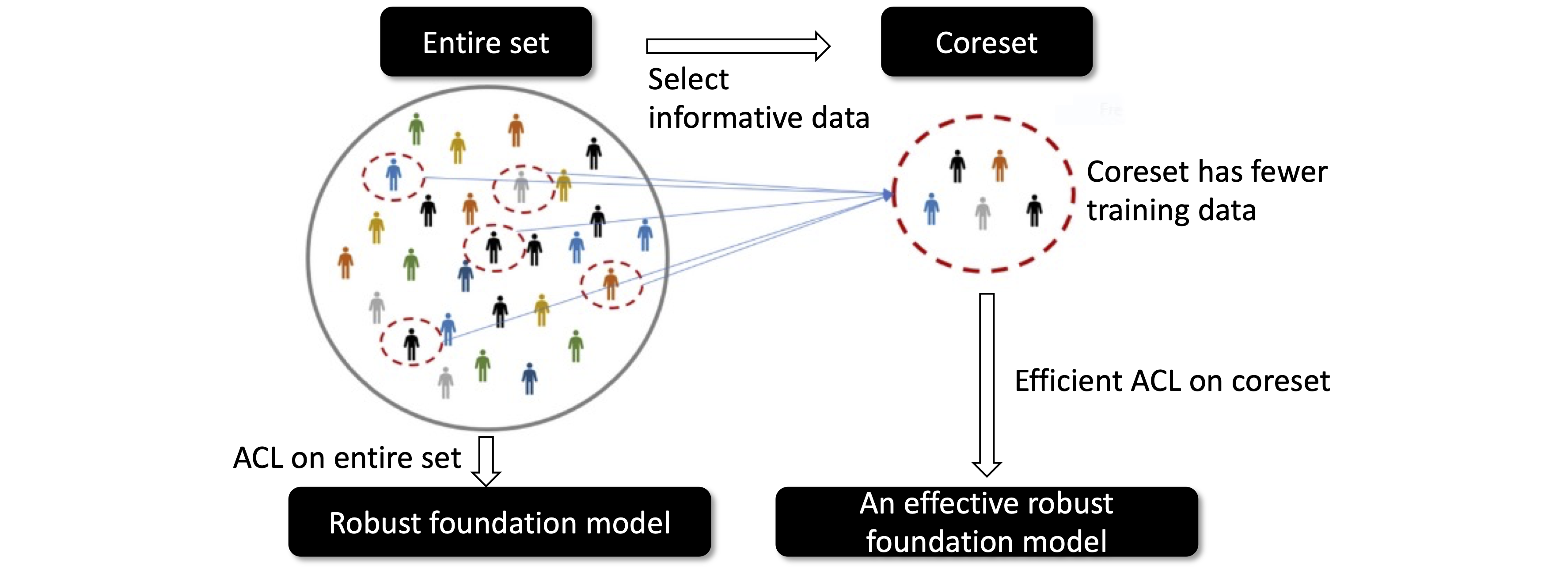
Representational Distance (RD) as a measurement of \(f\)’s adversarial robustness without labels.
RD of a data point \(\ell_\mathrm{RD}(x;\theta)\) is quantified by the representational distance between the natural data and its adversarial counterpart, i.e.,
\[\ell_{\mathrm{RD}}(x; \theta) = d(g \circ f_\theta(\tilde{x}), g \circ f_\theta(x)) \quad \mathrm{s.t.} \quad \tilde{x} = \mathop{\arg\max}_{x^{\prime} \in \mathcal{B}_\epsilon[x]} \quad d(g \circ f_\theta(x^{\prime}), g \circ f_\theta(x)),\]in which the PGD method is used to generate adversarial data \(\tilde{x}\) within the \(\epsilon\)-ball centered at \(x\) and \(d(\cdot, \cdot): \mathcal{V} \times \mathcal{V} \rightarrow \mathbb{R}\) is a distance function, such as the KL divergence. The smaller the RD is, the representations are of less sensitivity to adversarial perturbations, thus being more adversarially robust.
Objective function of RCS.
To realize the intuitive idea, RCS is formulated as follows:
\[S^* = \mathop{\arg\min}_{S \subseteq X, |S|/|X| = k} \mathcal{L}_{\mathrm{RD}}(U; \theta(S)),\] \[\theta(S) = \mathop{\arg\min}_{\theta} \mathcal{L}_\mathrm{ACL}(S; \theta),\]in which \(S^*\) is the coreset, \(U\) is an unlabled validation set, \(k \in (0,1]\) is subset fraction that controls the size of coreset, and \(\mathcal{L}_{\mathrm{RD}}(U; \theta(S)) = \sum_{x \in U} \ell_\mathrm{RD}(x; \theta(S))\), and \(\mathcal{L}_\mathrm{ACL}(S; \theta) = \sum_{x \in S} \ell_\mathrm{ACL}(x; \theta)\).
Intuitively, given a coreset \(S^*\), after the model parameters are updated to \(\theta(S^{*})\) via minimizing the ACL loss on the coreset \(\mathcal{L}_\mathrm{ACL}(S^*; \theta)\), the model will achieve the minimizied RD loss on the validation dataset \(\mathcal{L}_{\mathrm{RD}}(U; \theta(S^*))\), thus being adversarially robust.
Then, RCS can be converted into a problem of maximizing a set function subject to a cardinality constraint as follows:
\[S^* = \mathop{\arg\max}_{S \subseteq X, |S|/|X| = k} G_\theta(S),\] \[G_\theta(S \subseteq X) \triangleq - \mathcal{L}_\mathrm{RD}(U; \theta(S)) = - \mathcal{L}_\mathrm{RD}(U; \theta - \eta \nabla_\theta \mathcal{L}_\mathrm{ACL}(S; \theta)),\]where \(G:2^\mathcal{X} \rightarrow \mathbb{R}\) is a set function, \(\theta(S)\) is estimated using the one-step approximation and \(\eta \in \mathbb{R}^+\) is the learning rate.
RCS via Greedy Search.
The vanilla solution of traversing all subsets and selecting the subset that has the largest \(G_\theta(S)\) is intractable. Xu et al. (2023)
The set function \(G_\theta(S)\) is proved as submodular
- Monotonicity: As more data is added to the set, the representation becomes better.
\(G(x\mid X)=G(S \cup \{x\}) - G(S) \geq 0\) for any \(S \subseteq X\) and \(x \in X \setminus S\). - Diminishing returns: As the set has more data, the marginal gain of extra data for learning representations gradually diminishes.
\(\mathop{\forall}\limits_{A,B \mid A \subseteq B} G_\theta(x \mid A) \geq G_\theta(x \mid B)\).
Therefore, RCS greedily searches for the data \(x\) that has the largest marginal gain and then adds them into the coreset.
Pseudo-code of efficient ACL via RCS.
- Step 1 (Warm-up): Warm up training on the entire training set to find a better starting point \(f_\theta\).
- Step 2.1 (RCS): \(S \gets\emptyset\). \(\theta' \gets \theta\). Compute gradients \(Q \gets \{ q_k = \nabla_\theta \mathcal{L}_\mathrm{ACL}(x_k; \theta) \mid \forall x_k \in X \}\) on unlabeled training dataset \(X\).
- Step 2.2 (RCS): Compute gradients \(q_U \gets \nabla_\theta \mathcal{L}_\mathrm{RD}(U; \theta')\) on unlabeled validation dataset \(U\).
- Step 2.3 (RCS): Select a data \(x_k\), whose gradient \(q_k\) matches best with \(q_U\), i.e., \(\mathop{\arg\max}_k \{q_k^\top q_U \}\).
- Step 2.4 (RCS): \(S \gets S \cup \{x_k\}\), \(X \gets X \setminus \{ x_k \}\), \(\theta' \gets \theta' - \eta' q_k\).
- Step 2.5 (RCS): Repeat Steps 2.2-2.4 until \(\mid S\mid/\mid X\mid = k\).
- Step 3 (ACL training): Update parameters \(\theta \gets \theta - \eta \nabla_\theta \mathcal{L}_\mathrm{ACL}(S; \theta)\).
- Step 4: Every a few epochs, go to Step 2.1 to generate a new coreset; otherwise go to Step 3 to update model parameters. The algorithm stops when reaching the final training epoch.
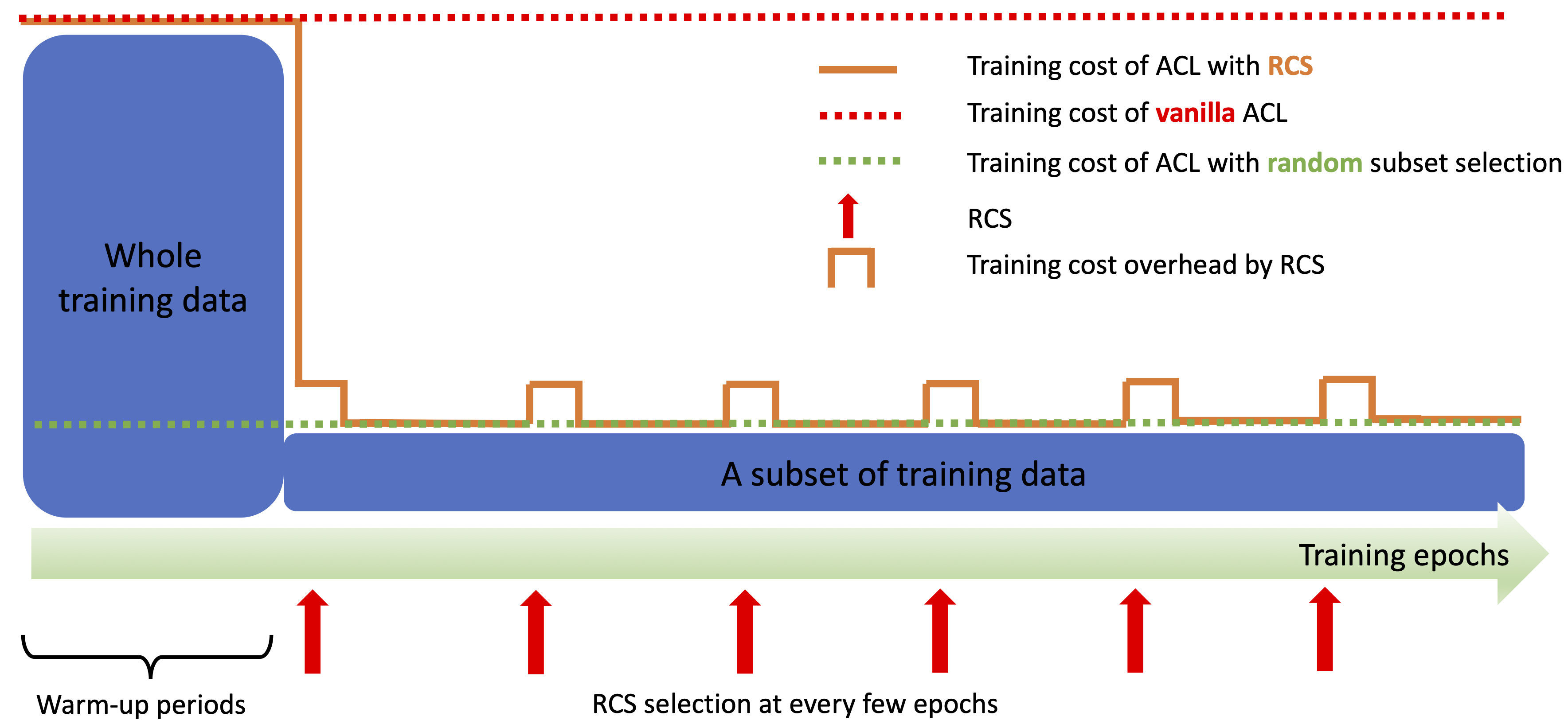
Intuitively, RCS greedily selects and adds the data \(x\) whose training loss gradient (i.e., \(\nabla_\theta\mathcal{L}_\mathrm{ACL}(\{x\}, \theta)\)) and validation loss gradient (i.e, \(\nabla_\theta\mathcal{L}_\mathcal{RD}(U; \theta(S))\)) have the most similarity into the coreset. In this way, training on the data selected by RCS is most beneficial in optimizing the RD loss, which is thus most helpful to improve \(f\)’s adversarial robustness.
The official code of RCS is available at https://github.com/GodXuxilie/Efficient_ACL_via_RCS.
Experimental Results
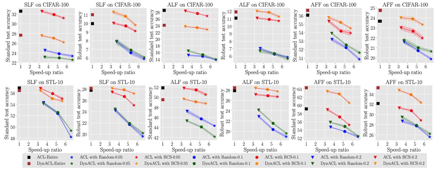
RCS significantly speeds up ACL on CIFAR-10.
- The term
speed-up ratiorefers to the ratio of the time consumption of pre-training on the training set to the the time consumption of pre-training on the training subset. Thus, the larger the speed-up ratio is, the more efficient the pre-training procedure is. - The terms
standard test accuracyandrobust test accuracyrefer to the average accuracy evaluated on natural test data and adversarial test data, respectively. Thus, the higher the line is, the more effective the pre-training method is.
The results obtained by RCS located in the upper-right corner is more efficient and more effective.
To reproduce the above results of the robustness transferability from CIFAR-10 to CIFAR-100, you can use the following scripts.
- At the pre-training stage, you can conduct ACL via RCS using ResNet-18 on CIFAR-10.
# Pre-training stage using RCS
git clone https://github.com/GodXuxilie/Efficient_ACL_via_RCS.git
cd Efficient_ACL_via_RCS/ACL_RCS/small_scale_datasets
PRE_TRAIN_DIR=ACL_RCS_ResNet18_cifar10
python DynACL_RCS.py $PRE_TRAIN_DIR --ACL_DS --dataset cifar10 --fraction 0.2- At the fine-tuning stage, you can fine-tune the pre-trained ResNet-18 on CIFAR-100. The test accuracy are saved in
$FINETUNE_DIR/results/log.txt.
# Fine-tuning stage (SLF, ALF, AFF)
cd Efficient_ACL_via_RCS/ACL_RCS/small_scale_datasets
PRE_TRAIN_DIR=ACL_RCS_ResNet18_cifar10
FINETUNE_DIR=ACL_RCS_ResNet18_cifar10_cifar100
python finetuning.py --experiment $FINETUNE_DIR \
                     --checkpoint ./checkpoints/$PRE_TRAIN_DIR/model.pt \
                     --dataset cifar100 \
                     --model r18 \
                     --mode ALL --eval-AA --eval-OOD --pretraining DynACL_RCS
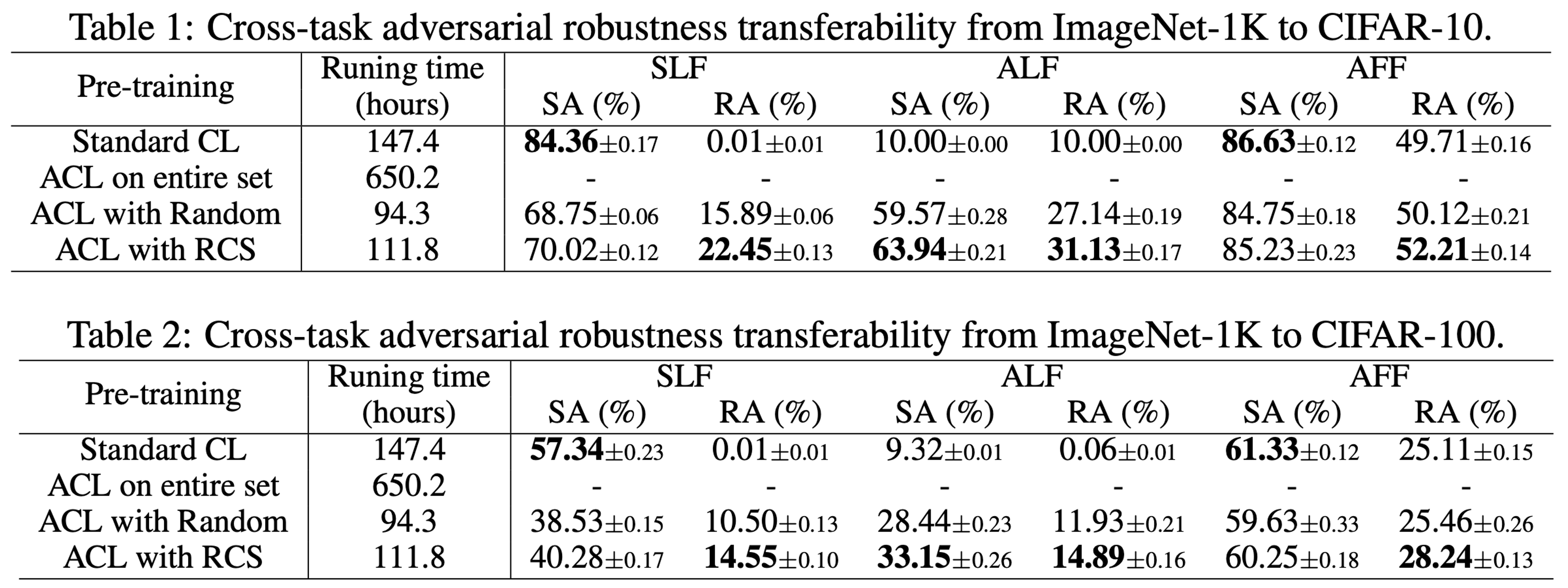
For the first time, ACL was conducted efficiently on ImageNet-1K via RCS. The results prove the possibility of applying ACL on large-scale datasets. Here, SA refers to standard test accuracy and RA refers to the robust test accuracy.
To reproduce the above results of the robustness transferability from ImageNet-1K to CIFAR-10, you can use the following scripts.
- At the pre-training stage, you can ACL via RCS using Wide ResNet with width 10 and depth 28 (WRN-28-10) on ImageNet-1K of \(32 \times 32\) resolution.
# Pre-training stage using RCS
git clone https://github.com/GodXuxilie/Efficient_ACL_via_RCS.git
cd Efficient_ACL_via_RCS/ACL_RCS/ImageNet_32
PRE_TRAIN_DIR=ACL_RCS_WRN_ImageNet
python ACL_RCS.py $PRE_TRAIN_DIR --gpu 0,1,2,3 --ACL_DS --fraction 0.05- At the fine-tuning stage, you can fine-tune the ImageNet-1K pre-trained models on CIFAR-10.
cd Efficient_ACL_via_RCS/ACL_RCS/ImageNet_32
PRE_TRAIN_DIR=ACL_RCS_WRN_ImageNet
FINETUNE_DIR=ACL_RCS_WRN_ImageNet_cifar10
# Fine-tuning stage (SLF)
python transfer.py --out_dir $FINETUNE_DIR/SLF \
                   --resume $PRE_TRAIN_DIR/model.pt
                   --dataset cifar10 \
                   --lr 0.01 --linear
# Fine-tuning stage (ALF)
python adv_tune.py --out_dir $FINETUNE_DIR/ALF \
                   --resume $PRE_TRAIN_DIR/model.pt \
                   --dataset cifar10 \
                   --lr 0.1 --linear
# Fine-tuning stage (AFF)
python adv_tune.py --out_dir $FINETUNE_DIR/AFF \
                   --resume $PRE_TRAIN_DIR/model.pt \
                   --dataset cifar10 \
                   --lr 0.1
RCS can speed up Standard Adversarial Training (SAT)

To reproduce the above results of the robustness transferability from ImageNet-1K to CIFAR-10, you can use the following scripts.
- At the pre-training stage, you can conduct SAT using WRN-28-10 on ImageNet-1K of \(32 \times 32\) resolution.
git clone https://github.com/GodXuxilie/Efficient_ACL_via_RCS.git
cd Efficient_ACL_via_RCS/SAT_RCS/ImageNet_32
# Pre-training stage using RCS
PRE_TRAIN_DIR=SAT_RCS_WRN_ImageNet
nohup python SAT_RCS.py --gpu 0,1,2,3 --out_dir $PRE_TRAIN_DIR --fraction 0.2- At the fine-tuning stage, you can fine-tune ImageNet-1K pre-trained WRN-28-10 on CIFAR-10.
cd Efficient_ACL_via_RCS/SAT_RCS/ImageNet_32
PRE_TRAIN_DIR=SAT_RCS_WRN_ImageNet
FINETUNE_DIR=SAT_RCS_WRN_ImageNet_cifar10
# Fine-tuning stage (ALF)
python adv_tune.py --out_dir $FINETUNE_DIR/ALF \
                   --resume $PRE_TRAIN_DIR/checkpoint.pth.tar \
                   --dataset cifar10 \
                   --lr 0.1 \
                   --linear
# Fine-tuning stage (AFF)
python adv_tune.py --out_dir $FINETUNE_DIR/AFF \
                   --resume $PRE_TRAIN_DIR/checkpoint.pth.tar
                   --dataset cifar10 \
                   --lr 0.1