The Hidden Convex Optimization Landscape of Two-Layer ReLU Networks
In this article, we delve into the research paper titled 'The Hidden Convex Optimization Landscape of Regularized Two-Layer ReLU Networks'. We put our focus on the significance of this study and evaluate its relevance in the current landscape of the theory of machine learning. This paper describes how solving a convex problem can directly give the solution to the highly non-convex problem that is optimizing a two-layer ReLU Network. After giving some intuition on the proof through a few examples, we will observe the limits of this model as we might not yet be able to throw away the non-convex problem.
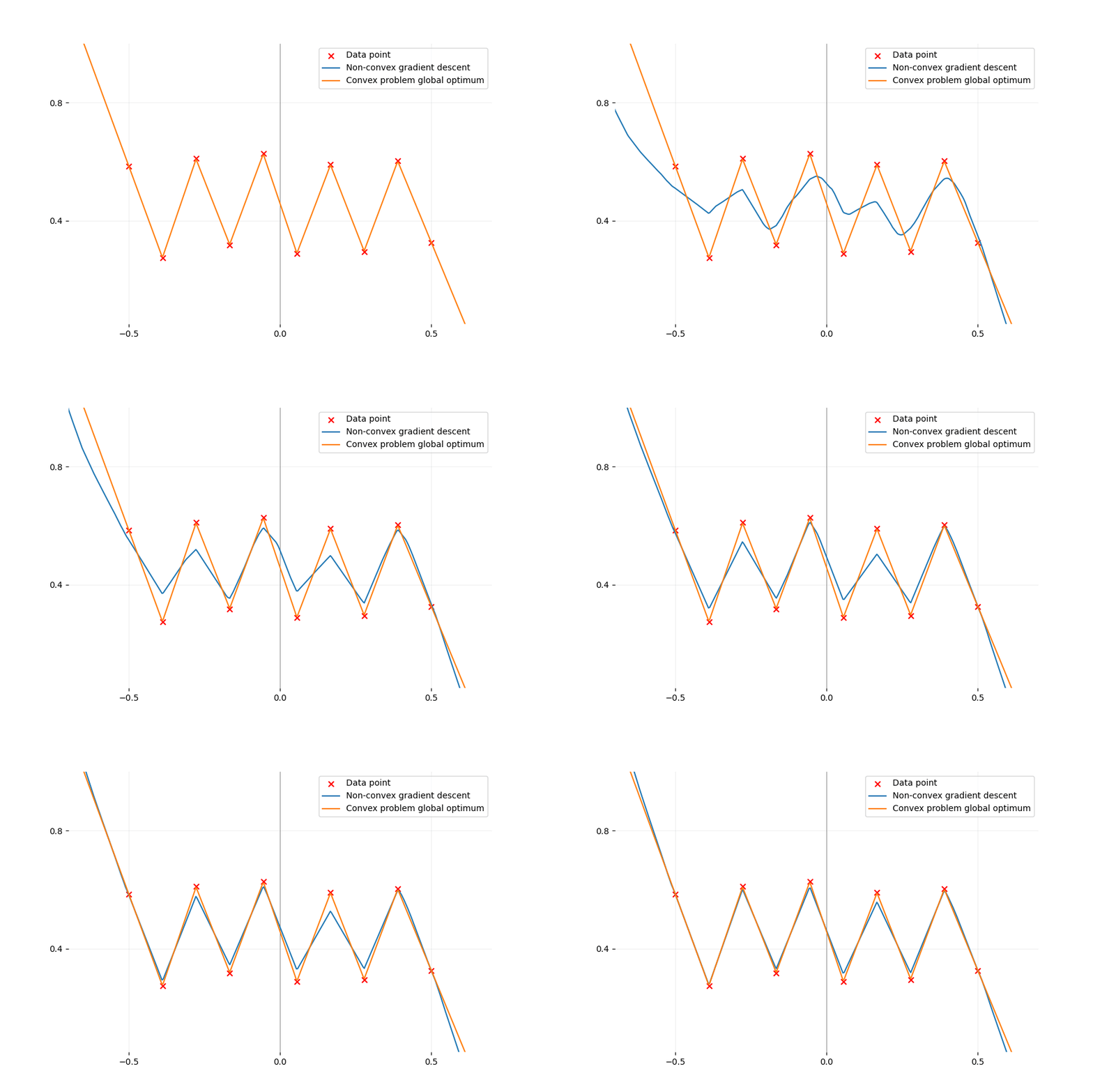
There exists an equivalent convex formulation to the classical non-convex ReLU two-layer network training. That sounds like great news but is it the case in practice? Let's find out together.
The code for this plot is available and reproducible on this Jupyter Notebook (or in HTML).
I. Overview and Motivation
50 years ago, two-layer networks with non-linear activations were known to be universal approximators, however, they did not catch on as they were hard to train. The recent years have been marked by deeper networks running on dedicated hardware with very large datasets. Those networks have since been at the top of the benchmark in many applications including self-driving and text generation. The pragmatic method to train such models is to run stochastic gradient descent on the non-convex optimization problem, which is concretely tuning the weights (and bias) until the model is accurate enough. The best models usually require billions of parameters and very large datasets. The training, in turn, requires millions of dollars of hardware and electricity to run gradient descent and train a single model.
Deep learning is not without faults. Even though the test performance can surpass those of many machine learning models, it is very hard to know what the network has learned because of its black-box nature. Interpretability in neural networks is crucial for creating trustworthy AI systems, one of the biggest obstacle to AI adoption. It may also lead us to simpler models that are cheaper to run, are more robust, generalize better, and are easier to adapt to specific tasks.
To figure out what a neural network learns, we will focus in this post on the training of a shallow ReLU network by vanilla gradient descent, using the full batch of data at each step, in a regression setting. More precisely, we will investigate how the construction of a convex equivalent to the non-convex training problem can enlighten us on how neurons evolve during the training phase, with a specific focus on the activation of the ReLU functions and their consequences.
Problem and notation
Our problem of interest will be the training of a simple two-layer neural network with ReLU activation. We focus on a classical regression problem with a mean squared error loss and we add a weight decay term (whose importance will be underlined later). This leads to the following full-batch gradient method (note that we make a slight abuse of notation by denoting by $\nabla$ the output of the derivative of the parameters, obtained, for instance, by backpropagation).
Because there are only two layers, we will integrate the biases of the neurons directly into the data by adding a dimension filled with ones.
Two-Layer ReLU Network Training
Data points: $n$ inputs \(\pmb{x}_j \in \RR^d\) and labels \(y_j \in \RR\), $j=1,..,n$
Model: $m$ neurons: First layer \(\pmb{w}_i \in \RR^d\), second layer \(\alpha_i \in \RR\), $i=1,..,m$
Hyper-parameters: step-size \(\step > 0\), regularization \(\lambda\geq 0\)
Loss to be minimized: \begin{equation}\label{eq:theloss} \mathcal{L}(\pmb{W}, \pmb{\alpha}) = \sum_{j=1}^n \bigg( \underbrace{\sum_{i=1}^m \max(0, \pmb{w}_i^\top \pmb{x}_j) \alpha_i}_{\text{Network's Output}} - y_j \bigg)^2 + \underbrace{\lambda \sum_{i=1}^m \| \pmb{w}_i \|^2_2 + \alpha_i^2}_{\text{Weight Decay}} \end{equation} (Full-batch) Gradient Descent: \begin{equation*} (\pmb{W}, \pmb{\alpha})_{t+1} = (\pmb{W}, \pmb{\alpha})_t - \step \nabla \mathcal{L}((\pmb{W}, \pmb{\alpha})_t) \end{equation*}
Even the simplest ReLU models have non-trivial non-convexity as depicted in the figure below. We plot the loss function \(\mathcal{L}\) of a network with two neurons on one-dimensional data. We only optimize the first layer here so we have a total of two parameters to optimize. Despite the simple setup, a gradient descent starting from a random initialization can converge to three different values, two of them being bigger than zero. However, there always exists a path of non-increasing loss from initialization to the global minimum (as predicted by a
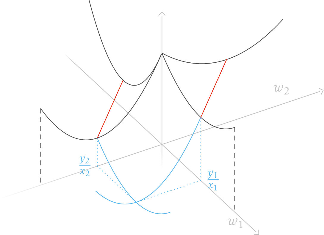
Loss landscape of a network with two parameters, one for each ReLU neuron, and two data points: $(x_1, y_1) = (-1, 1)$ and $(x_2, y_2) = (1, 2)$ are fixed. Since all labels are positive, we fix the second layer $\alpha_1, \alpha_2$ to 1 to plot the loss in 2D without a loss of generality. The black lines represent the loss for only one neuron (since the other is equal to 0). The red lines(critical points) are paths of parameters for which the loss is constant and the gradient is zero. They represent the parameters for which the neuron fits exactly one data point and is deactivated for the other and thus suffers a loss of $(y_1)^2$ for the red line on the left and $(y_2)^2$ for the other. The exact formula to compute each point of the loss landscape is: \begin{equation*} \begin{split} \mathcal{L}(w_1, w_2) =&\ \left(\max(0, x_1 w_1) + \max(0, x_1 w_2) - y_1\right)^2 \\ +&\ \left(\max(0, x_2 w_1) + \max(0, x_2 w_2) - y_2\right)^2 \end{split} \end{equation*}
To avoid the local minima, one idea is to add constraints to the parameters. The constrained problem where $w_1$ has to be positive and $w_2$ has to be negative, is convex, and a simple gradient descent will find the global minima of the original unconstrained problem. In
In this blog post, we will first work out the intuition needed to understand why an equivalent, finite convex problem even exists. Then we will study the exact links between the problem in practice and the convex problem, and go over the limits of such an approach both in theory and in practice.
Research context
The question of how neural networks learn is a very active domain of research with many different paths of investigation. Its main goal is to lay a mathematical foundation for deep learning and for that goal, shallow neural networks act as a stepping stone for understanding deeper and more complex networks.
For networks with a hidden layer of infinite width, it is proven that gradient descent converges to one of the global minima
Examining the loss landscape reveals that shallow networks with more neurons than data points always have a non-increasing path to a global minimum
Regularization plays a pivotal role as it let us influence which local minimum we will reach with gradient descent, usually to favor a simpler solution. Even if no explicit regularization is used, it is known that there is an implicit bias of gradient descent for linear activations, and more recently for ReLU networks
Other convex approaches are limited to an infinite amount of neurons, or to optimization in neuron-by-neuron fashion
To sum up, the convex reformulation approach described in this post contrasts with what precedes by presenting results for a shallow network with finite width layers, in a regression setting with ReLU activation and weight decay regularization.
II. Convex reformulation
Small example walkthrough
First, let’s get familiar with and understand the inherent convexity caused by ReLU and the second layer. To do so, we will take simple yet non-convex examples and find their global minima using a convex problem.
One ReLU, no second layer, no regularization
Below is the loss of a single ReLU neuron (\(w_1 \in \RR\)) trained on two data points: \((x_1, y_1)=(-1, 1)\) and \((x_2, y_2) = (1, 0.5)\)
\begin{equation}\label{eq:one_neuron_loss} {\color{cvred}{\mathcal{L}}}(w_1) = \big(\max(0, x_1 ~ w_1) - y_1\big)^2+\big(\max(0, x_2 ~ w_1) - y_2\big)^2 \end{equation}
Because our only trainable parameter is one-dimensional, we can directly plot the entire loss landscape.

\(\color{cvred}{\mathcal{L}}\) is non-convex in a strong sense: two local minima exist and have distinct values (\((y_1)^2\) and \((y_2)^2\)). In practice, a gradient descent will never be able to switch from fitting one data point to the other (switching from positive to a negative weight $w_1$ can only be done by increasing the loss).
We say that the ReLU neuron can activate one or more data points if the output of its ReLU is non-zero when evaluated on said data. The output of a one-neuron ReLU network is \(\color{cvblue}{\max(0, x ~ w_1)}\), we can plot both the output and the two data points on the same graph.
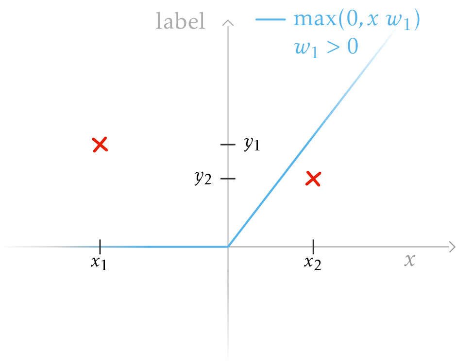
Plot of the output of a one-neuron ReLU network with a positive weight $w_1$. The ReLU only activates the second data point (as $x_2>0$ and $w_1 > 0$) so the network can fit the second data point. However, doing so means it cannot activate $x_1$ and will incur a constant loss $(y_1)^2$. Overall, depending on the sign of $w_1$, we will have a loss consisting of a constant term for not activating one example and a quadratic term for matching the label of the activated data point.
Before moving on, the important fact here is that we have a true non-convexity of the loss(the difference between two local minima $\vert (y_1)^2 - (y_2)^2 \vert$ can be made arbitrarily large), even without a single layer or regularization. Now we will explore the corresponding convex problems.
Activation
We want to find the global minima of the one-neuron ReLU network loss function\eqref{eq:one_neuron_loss}. Recall that the loss has two local minima: $(y_2)^2$ for $w_1=y_1/x_1$ and $(y_1)^2$ for $w_1=y_2/x_2$.
Which data points are activated plays a crucial role in the loss. In the specific example above, $x_2>0$ is activated and $x_1<0$ is not. If we fix the ReLU’s activation to this pattern and replace the max operators with \(\czero\) or \(\cone\):
\begin{equation}\label{eq:firsttry} \min_{u_1 \in \RR} (\czero \times x_1 u_1 - y_1)^2+ (\cone \times x_2 u_1 - y_2)^2 \end{equation}
This problem is convex. A gradient descent from any initialization will converge to the optimal loss $(y_1)^2$ with the parameter $u_1 =y_2/x_2$. This parameter directly corresponds to one of the two local minima of the non-convex loss\eqref{eq:one_neuron_loss} by taking $w_1 = u_1$.
\begin{equation*} \min_{u_2 \in \RR} (\cone \times x_1 u_2 - y_1)^2+ (\czero \times x_2 u_2 - y_2)^2 \end{equation*}
Similarly, this convex problem’s optimal solution directly corresponds to the second local minima: $(y_2)^2$ for $u_2 =-y_1/x_1$.
All seems good. But keep in mind that we want to build an equivalent problem. If $u_2$ is positive, taking $w_1 = u_2$ does not lead to the same loss value in the original problem because a positive parameter will never activate the first data point.
To make the issue obvious, consider this convex problem obtained by replacing the two $\max$ operators by \(\cone\):
\begin{equation*} \min_{u_3 \in \RR} (\cone \times x_1 u_3 - y_1)^2+ (\cone \times x_2 u_3 - y_2)^2 \end{equation*}
While it is convex, there is no link between the ReLU parameter $w_1$, and this new problem’s parameter $u_3$: it is not possible to activate both data points. This issue comes from the fact that replacing a $\max$ by \(\cone\) only makes sense if what is inside the $\max$ is indeed positive. In other words, as long as \(x_1 ~ w_1\) is positive we have that \(max(x_1 ~ w_1, 0) = \cone x_1 ~ w_1\).
\begin{equation*} \min_{\substack{x_1 ~ u_3 \geq 0\\x_2 ~ u_3 \geq 0}} (\cone \times x_1 u_3 - y_1)^2+ (\cone \times x_2 u_3 - y_2)^2 \end{equation*}
We added the constraints corresponding to the activation, and it adequately restricts $u_3$ to be in ${0}$.
As a simple reformulation of \eqref{eq:firsttry}, we vectorize (in the number of data points) the convex loss and we add the constraints:
\begin{equation*} \min_{\substack{\begin{bmatrix}-1 & 0 \\ 0 & 1\end{bmatrix} \begin{bmatrix} x_1 \\ x_2 \end{bmatrix} u_1 \geq 0}} \ \ \bigg\| \underbrace{\begin{bmatrix} \czero & 0 \\ 0 & \cone \end{bmatrix}}_{\text{diagonal activation matrix}} \begin{bmatrix} x_1 \\ x_2 \end{bmatrix} u_1 - \begin{bmatrix} y_1 \\ y_2 \end{bmatrix} \bigg\|_2^2 \end{equation*}
The diagonal activation matrix (named \(D_i \in \{0, 1\}^{n \times n}\)) summarize the on/off behavior of one ReLU for all data points. The constraints on $u_1$ are directly given by this activation matrix:
\[\begin{bmatrix} -1 & 0 \\ 0 & 1 \end{bmatrix} = 2 \begin{bmatrix} \czero & 0 \\ 0 & \cone \end{bmatrix}- I_2 \qquad \text{$I_2$ the identity matrix of $\RR^2$}\]The other way around, we can define the activation pattern vector for a specific parameter \(u\): \((\mathbb{1}_{u ~ x_j \geq 0})_{j=1\dots n} \in \{0,1\}^n\) with $n$ the number of data points. The activation matrix of \(u\) is simply the matrix that has this vector for its diagonal.
So we have exactly four possible activation matrices. \(D_1 = (\begin{smallmatrix} \czero & 0 \\ 0 & \czero \end{smallmatrix})\) and \(D_2 = (\begin{smallmatrix} \cone & 0 \\ 0 & \cone \end{smallmatrix})\) will have constraints that reduce to $w_1 = 0$, making them not interesting. The other two lead to convex problems with convex constraints. Solving them will give the parameters that correspond to the two local minima of the loss of ReLU neural network with only a single neuron\eqref{eq:one_neuron_loss}.
For any number $n$ of 1-D data points, there are $2^n$ distinct activation matrices but only two of them will be interesting: activating all positive data points, or only activating negative data points. Only some $D_i$ are interesting in higher dimensions, but finding all of them is not obvious.
Replacing everything with the usual matrices (\(X=(\begin{smallmatrix}x_1 \\x_2\end{smallmatrix})\), \(Y=(\begin{smallmatrix}y_1 \\y_2\end{smallmatrix})\)) will get us the equivalent convex problem to a one-neuron ReLU network, whose activation pattern is $D_i$:
\begin{equation*} \min_{\substack{u_1 \in \RR\\ (2 D_i - I_2) X u_1 \geq 0}} \ \ \big\| D_i X u_1 - Y \big\|_2^2 \end{equation*}
Later sections will investigate what we can say about a ReLU network with more than one neuron.
Multiplicative non-convexity from the second layer

\begin{equation}\label{eq:ncvxlin} \min_{(x, y) \in \RR^2} (x ~ y - 1)^2 \end{equation}
\eqref{eq:ncvxlin} is not convex, it has two local minima. However, they are symmetric. Simply replace the term $x ~ y$ by a new variable $z$, and use a simple mapping such as $z \rightarrow (1, z)$ to get the solution of \eqref{eq:ncvxlin} from the solution of the convex problem: \(\min_{z \in \RR} (z-1)^2\).
The initial problem\eqref{eq:ncvxlin} with L2 regularization is non-convex as well:
\begin{equation*} \min_{(x, y) \in \RR^2} (x ~ y - 1)^2 + \frac{\lambda}{2} ( \vert x \vert^2 + \vert y \vert^2) \end{equation*}
The convex reformulation with one variable is:
\begin{equation*} \min_{z \in \RR} (z - 1)^2 + \lambda \vert z \vert \end{equation*}
We have to use a different mapping \(z \rightarrow (\sgn(z) \sqrt(\vert z \vert), \sqrt(\vert z \vert))\). One can verify that plugging this mapping into the non-convex problem will give the same value. Therefore, you can solve the convex problem in lieu of the non-convex one.
Back to non-linear activations, consider the non-convex problem of training a single ReLU neuron with a second layer(\(\alpha_1\)) and a L2 regularization:
\begin{equation*} \min_{(w_1, \alpha_1) \in \RR^2} \big(\max(0, x_1 w_1) \alpha_1 - y_1\big)^2 + \frac{\lambda}{2} \left(\vert w_1 \vert^2 + \vert \alpha_1 \vert^2\right) \end{equation*}
We fix the activation to only activate $x_1$(as could be done for any activation pattern) and add the corresponding constraint as done in the previous section:
\begin{equation}\label{eq:ncvx1} \min_{\substack{(u_1, \alpha_1) \in \RR^2\\ x_1 ~ u_1 \geq 0}} \left( \cone ~ x_1 ~ u_1 ~ \alpha_1 - y_1 \right)^2 + \frac{\lambda}{2} (\vert u_1 \vert^2 + \vert \alpha_1 \vert^2) \end{equation}
\eqref{eq:ncvx1} is a non-convex problem because we are multiplying $w_1$ and $\alpha_1$ together (and some constant). However, this non-convexity can be ignored by considering an equivalent convex function in a very similar way to the $(x ~ y - 1)^2$ problem.
\begin{equation}\label{eq:cvx1} \min_{x_1 ~ z_1 \geq 0} \left( \cone ~ x_1 ~ z_1 - y_1 \right)^2 + \lambda \vert z_1 \vert \end{equation}
$z_1$ takes the role of the product $w_1 ~ \alpha_1$. We can solve \eqref{eq:cvx1} to get an optimal $z_1$ and then use a mapping \((w_1, \alpha_1) = (\sgn(z_1) ~ \sqrt{\vert z_1 \vert}, \sqrt{\vert z_1\vert})\). However, the two problems do not have the same expressivity: \(\max(0, x_1 ~ z_1) \alpha_1\) can be negative but not \(\cone ~ x_1 ~ z_1\) because of the constraint. Let’s add a second variable with the same constraint as $z_1$ that will take the role of a negative $\alpha_1$.
\begin{equation}\label{eq:cvx2} \min_{\substack{x_1 ~ z_1 \geq 0\\x_1 ~ v_1 \geq 0}} \big( \cone ~ x_1 ~ (z_1 - v_1) - y_1 \big)^2 + \lambda (\vert z_1 \vert + \vert v_1 \vert) \end{equation}
The variable \(z_1\) represents a neuron with a positive second layer and \(v_1\) a neuron with the same activation pattern but with a negative second layer. This is a convex problem(adding a convex regularization preserves the convexity) with convex constraints. At the optimum, only one of the two variables will be non-zero. We consider this mapping:
\begin{align*} (w_1, \alpha_1) &= (\sgn(z_1) ~ \sqrt{\vert z_1 \vert}, \sqrt{\vert z_1 \vert}) & \text{ if $z_1$ is non-zero}\\ (w_1, \alpha_1) &= (\sgn(v_1) ~ \sqrt{\vert v_1 \vert}, - \sqrt{\vert v_1 \vert}) & \text{ if $v_1$ is non-zero} \end{align*}
One can verify that this mapping does give the same value when plugged into \eqref{eq:ncvx1}. The two problems share the same global minima as we can easily map back and forth without altering the loss. The global minima of the two problems have the same value as they have the same expressivity, we can say the two problems are equivalent in the sense that we can solve one to get the solution of the other by a simple mapping.
To summarize, here’s the equivalent (with the above mapping) convex problem for a one-neuron ReLU Network with regularization and a second layer, whose activation pattern is $D_i$:
\begin{equation*} \min_{\substack{(2 D_i - I_2) X u_1 \geq 0\\ (2 D_i - I_2) X v_1 \geq 0}} \ \ \big\| D_i ~ X (u_1 - v_1) - Y \big\|_2^2 \end{equation*}
Equivalent Convex problem with two neurons
Before moving on to the general results, we want to fit two data points, i.e. having both data points activated. To do so, we need at least two neurons. The usual non-convex problem is as follows (with \(X=(\begin{smallmatrix}x_1 \\x_2\end{smallmatrix})\), \(Y=(\begin{smallmatrix}y_1 \\y_2\end{smallmatrix})\) and $m=2$):
\begin{equation*} \min_{w_i, \alpha_i \in \RR, i=1 \dots m} \bigg\| \sum_{i=1}^m \max(0, X w_i) \alpha_i - y \bigg\|^2_2 + \lambda \sum_{i=1}^m w_i ^2 + \alpha_i^2. \end{equation*}
This loss is plotted (with $\lambda = 0$ and fixed second layer) in the introduction section. The convex reformulation is very similar.
\begin{equation*} \min_{\substack{(2 D_i - I_2) X u_i \geq 0\\ (2 D_i - I_2) X v_i \geq 0}, i=1 \dots m} \ \ \bigg\| \sum_{i=1}^m D_i ~ X (u_i - v_i) - Y \bigg\|_2^2 + \lambda \sum_{i=1}^m \vert u_i \vert +\vert v_i \vert \end{equation*}
The best choice(only obvious in this 1-D data case) of activation matrices would be \(D_1 = (\begin{smallmatrix} \czero & 0 \\ 0 & \cone \end{smallmatrix})\) and \(D_2 = (\begin{smallmatrix} \cone & 0 \\ 0 & \czero \end{smallmatrix})\).
Solving and mapping the solutions would give the optimal global solution to the problem of fitting two data points with a ReLU network with two neurons. More insights about why this is true are given after the general case section, and the complete proof can be found in the paper.
General Case
Let us consider a general two-layer ReLU network with an input of dimension $d$, an output of dimension 1 (vector output requires a similar but parallel construction
\begin{equation*} \mathcal{L}(\pmb{W}, \pmb{\alpha}) = \bigg\| \sum_{i=1}^m \max(0, \pmb{X} \pmb{w}_i) \alpha_i - \pmb{y} \bigg\|^2_2 + \lambda \sum_{i=1}^m \| \pmb{w}_i \|^2_2 + \alpha_i^2 \end{equation*}
This is the same loss as presented at the beginning of the article\eqref{eq:theloss} but with matrix and vectors. \(\pmb{X} \in \RR^{n \times d}\) is the data matrix and \(\pmb{y} \in \RR^n\) are the labels. Each neuron has its first layer parameter \(\pmb{w}_i \in \RR^d\) and second layer \(\alpha_i \in \RR\).
By analogy with what we saw earlier, an equivalent convex problem can be found. Multiplications are replaced by scalar products in the definition of activation matrices and thus most insights about activation hold.
\begin{equation}\label{eq:thecvx} \min_{\pmb{U}, \pmb{V} \in \mathcal{K}} \bigg\| \sum_{i=1}^m \pmb{D}_i \pmb{X} (\pmb{u}_i - \pmb{v}_i) - \pmb{y} \bigg\|^2_2 + \lambda \sum_{i=1}^m \| \pmb{u}_i \|_2 + \| \pmb{v}_i \|_2 \end{equation}
\(\pmb{D}_i\) are the activation matrix. The set of the constraints \(\mathcal{K}\) is the concatenation of the constraints of all neurons. Each constraint can be written succintely: \((2 \pmb{D}_i - \pmb{I}_n) X \pmb{u}_i \geq 0\). If \(u_i\) respects the constraint, its activation pattern is exactly \(D_i\) and this is crucial to retrieve the optimal solution of the non-convex loss\eqref{eq:theloss} from the solution of the convex reformulation\eqref{eq:thecvx}.
A conceptually easy way to have the two problems have the same global loss, is to consider a ReLU network with \(2^n\) neurons, and to formulate the convex problem using all \(2^n\) distinct activation matrices \(D_i\). In that case, it is easy to see that they both have the same expressivity. In the paper, it is proved that in theory only \(n\) neurons and activation patterns are required (using carathéodory’s theorem), but the patterns are not given explicitly. The next section will give more insights on when the two problems are equivalent.
From a solution of the convex problem\eqref{eq:thecvx}, the convex neurons \(u_i\) can be mapped to the non-convex neurons \((w_i, \alpha_i)\) using this mapping:
\begin{align*} (w_i, \alpha_i) &= (\frac{u_i}{\sqrt{\| u_i \|_2}}, \sqrt{\| u_i \|_2}) & \text{ if $u_i$ is non-zero}\\ (w_i, \alpha_i) &= (\frac{v_i}{\sqrt{\| v_i \|_2}}, -\sqrt{\| v_i \|_2}) & \text{ if $v_i$ is non-zero} \end{align*}
We use the same mapping as in the 1D case except the direction of the neuron (\(u_i\)) is now a vector in \(\RR^d\)
This is a very simple mapping from convex solution to non-convex neurons. We will call convex neurons the set of parameters that correspond to a neuron in the original, non-convex problem. One can expect similar trajectories between the non-convex and convex neurons during gradient descent.
Here, we fixed the number of neurons and the corresponding activations. A few questions are left unanswered: how many different activation patterns need to be considered, and how many neurons should we consider for both convex and non-convex problems?
Specifics about equivalence
Two problems are considered equivalent when their global optima can be seamlessly mapped back and forth.
As seen before, there are only two interesting possible activation patterns in the one-dimensional case (a single neuron can either activate all the positive data points and none of the negative, or the opposite), but there are close to \(2^n\) interesting patterns when the data dimension is higher. An activation pattern is interesting if there exists a non-zero vector that can respect the constraints and in fine, the activation pattern.
The (unique) optimal loss of the convex problem \eqref{eq:thecvx} with all possible activation patterns(for fixed data) \(D_i\) is the best loss any non-convex network can reach. The following sections are dedicated to understanding why adding more neurons than there are activation patterns will not improve the loss.
However, if we only consider a subset of all patterns, the convex problem will in general correspond to a local optimum of the non-convex network. Indeed, it is not as expressive as before. This would either correspond to a non-convex network with not enough neurons, or with too many neurons concentrated in the same regions.
To explore this idea, we go back to one-dimensional data.
1-D EXAMPLE, ONE NEURON
In the non-convex problem with only one neuron, there are exactly two local minima.
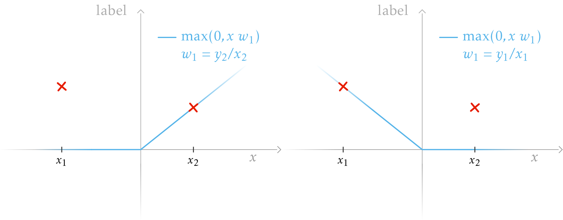
Plot of the output of a ReLU Network with one neuron, one for each of the parameter's local minima. The parameter on the left can be formulated as a solution of a convex problem with one convex neuron using the activation matrix \((\begin{smallmatrix} \czero & 0 \\ 0 & \cone\end{smallmatrix})\), and \((\begin{smallmatrix} \cone & 0 \\ 0 & \czero \end{smallmatrix})\) for the right output.
As seen in the previous section, each local minimum can be found exactly by solving the convex problem with a subset of all possible activations, that is on the left and on the right. Here we cannot say that the convex problem (that considers only one pattern) is equivalent to the non-convex one because the global minimum of the non-convex cannot be achieved in the convex problem. However, once we reach a local minimum in the non-convex gradient descent, then it can be described as a convex problem, by considering one pattern or the other.
1-D EXAMPLE, TWO NEURONS

The non-convex problem initialized with two random neurons and optimized with gradient descent will have three possible local minima (if there is some regularization, otherwise there's an infinite number of them). Either we initialize a neuron for each activation and it will reach the global optima (left), or two of them will end up in the same pattern (right), activating the same data point.
In the case of two neurons, the convex equivalent problem is as follows:
\begin{equation*} \mathcal{L}(u_1, u_2)= \bigg\| \begin{bmatrix} \czero & 0 \\ 0 & \cone \end{bmatrix} \begin{bmatrix} x_1 \\ x_2 \end{bmatrix} u_1 + \begin{bmatrix} \cone & 0 \\ 0 & \czero \end{bmatrix} \begin{bmatrix} x_1 \\ x_2 \end{bmatrix} u_2 - \begin{bmatrix} y_1 \\ y_2 \end{bmatrix} \bigg\|_2^2 + \lambda (| u_1 | + | u_2 |) \end{equation*}
is equivalent to the non-convex problem i.e. solving it will give the global optimum of the non-convex objective. (the negative $v_i$ are zero at the optimal and are removed here only to be clear.)
1-D EXAMPLE, MANY NEURONS

Plotting the positive part of many ReLU neurons. Summed up, they form a network output that perfectly fits the data.
We draw one example of a usual local minimum for gradient descent in the specific case of having more neurons than existing patterns. In practice (with more data in higher dimensions) there are much fewer neurons than possible activations. However, there are many situations in which neurons will lead to the same activation patterns, and in the experiment section we will see how to force such dynamics.
Note that we can merge neurons that are in the same activation pattern by summing them up (even in higher dimensions), creating a new neuron, and keeping both the output and the loss unchanged (although regularization might decrease). The fact that having more than one neuron in one pattern does not decrease the loss is at the core of the proof.
Activation patterns
The equivalence proof is heavily based on ReLU, specifically that a ReLU unit divides the input space into two regions: one where it will output zero, and the other where it is the identity. If you consider a finite set of samples and a single ReLU, it will activate and deactivate some samples: this is called an activation pattern. A diagonal matrix \(\pmb{D}_i \in \{0,1\}^{n \times n}\) describes one activation pattern, but not all are possible for a given dataset. There is a finite amount of such possible patterns, exponential in the dimension of the data.
This section is important to understand the final animations in the experimental section and helps understand how active activation patterns evolve in the non-convex problem.
Two-Dimensional Data
In the previous part, we considered data to be one-dimensional which resulted in only two possible activation patterns. Let us consider two-dimensional data. To do so in the simplest way possible, we will consider regular one-dimensional data and a dimension filled with \(1\)s. This will effectively give the neural network a bias to use without modifying the formulas.
We consider two data points: \(\color{cvred}{\pmb{x}_1} = (-0.2, 1)\) and \(\color{cvred}{\pmb{x}_2} = (1, 1)\), each associated with their label \(y_1 = 0.5\) and \(y_2 = 1\). We plot the output of one ReLU unit initialized at \(\pmb{w}_1 = (0.3, 0.15)\), \(\alpha_1 = 1\). Therefore we have
\begin{align*} \max(0, \pmb{w}_1^\top \pmb{x}_1) &= 0 \\ \max(0, \pmb{w}_1^\top \pmb{x}_2) &= \pmb{w}_1^\top \pmb{x}_2 \end{align*}
The activation pattern of \(\pmb{w}_1\) is \(\pmb{D}_1=\left(\begin{smallmatrix} \czero & 0 \\ 0 & \cone \end{smallmatrix}\right)\). There are only three other possible activation patterns, activating both data points: \(\pmb{D}_2=\left(\begin{smallmatrix} 1 & 0 \\ 0 & 1 \end{smallmatrix}\right)\), activating only the first one with \(\pmb{D}_3=\left(\begin{smallmatrix} 1 & 0 \\ 0 & 0 \end{smallmatrix}\right)\) and activating no data point with a zero matrix.
One point of interest is the data for which the ReLU will be 0. This is where the output changes its slope: \(a_1 = -w_1^2/w_1^1\) where \(w_1^i\) is the i-th coordinate of \(\pmb{w}_i\). Here, \(a_1 = 0.5\). We call this the activation point of the neuron \(\pmb{w}_1\).
We plot the output, \(\color{cvblue}{\max(0, (x, 1) ~ \pmb{w}_1^\top)}\), of the network as a function of the first dimension of the data \(x^1\) (here simply written \(x\)):

A neuron initialized so that it activates only one data point i.e. its activation point is between the two samples, and its slope tells us if it activates on the left or on the right like in this case.
Illustration.
In the animation below, we train this network using vanilla gradient descent on the two data points \(\color{cvred}{\pmb{x}_1}\) and \(\color{cvred}{\pmb{x}_2}\), represented by the red crosses. We plot its \(\color{cblue}{\text{output}}\) in blue for every possible data point (omitting the second dimension as it is always 1 in this example, playing the role of the bias), and we plot in red the label associated with the two data points. Each frame corresponds to one step of full-batch gradient descent with a small learning rate. We mark the \(\color{cgreen}{\text{activation point}}\) of the neuron with a green triangle, pointing toward the side the neuron activates. The green triangle’s height is the slope of the ReLU’s output, equal to \(u_1^1 = w_1^1 \alpha_1\), allowing us to visualize how important one neuron is for the output of the network.
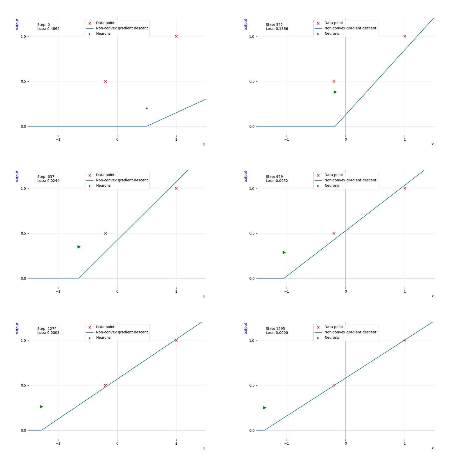
Training a single neuron network with gradient descent until it exactly fits two data points. It starts by fitting the only point it activates, \(\color{cvred}{\pmb{x}_2}\). As training progresses, the activation point represented by a green triangle shifts position. As soon as the activation point reaches \(\color{cvred}{\pmb{x}_1}\), it activates it and starts fitting both points at the same time. Its activation pattern shifts from \(\left(\begin{smallmatrix} \czero & 0 \\ 0 & \cone \end{smallmatrix}\right)\) to \(\left(\begin{smallmatrix} \cone & 0 \\ 0 & \cone \end{smallmatrix}\right)\) and stays the same until convergence.
Adding more neurons will not create additional activation patterns, only adding more data points will. With only two data points \(\pmb{x}_1\) and \(\pmb{x}_2\), we only had 4 possible patterns, with four data points we have 10 possible patterns.
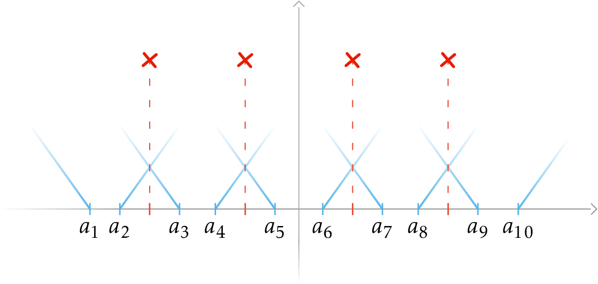
We plot the individual output and activation points of each of the ReLU neurons associated with the ten _interesting_ activation patterns in blue. Those are the 10 (20 with negative ones) neurons that need to be considered to get the global optima using the convex equivalent. When moving the activation point \(a_i\) of a neuron between two data points, its activation pattern does not change.
Notice that it is not possible to only activate the data points in the middle. However, if we increase the data's dimension, this becomes possible. This is also possible with a second layer of ReLU. In higher dimensions, we cannot visualize the activation patterns as easily, but we can understand that as dimensionality increases, more patterns are possible as it is easier to separate different data points.
Extensions of the convex reformulation to other settings
Batch Normalization (BN) is a key process that adjusts a batch of data to have a mean of zero and a standard deviation of one, using two trainable parameters. In the convex equivalent, we replace \(\pmb{D}_i \pmb{X}\) with \(\pmb{U}_i\). This \(\pmb{U}_i\) is the first matrix in the Singular Value Decomposition (SVD) of \(\pmb{D}_i \pmb{X} = \pmb{U}_i \pmb{\Sigma}_i \pmb{V}_i\)
III. Can We Forget the Non-Convex Problem?
Solving the convex problem efficiently is hard
In the last ten years, deep neural networks have been trained using (stochastic) gradient descent on the non-convex problem. The algorithm, the implementation, and even the hardware running the training have been heavily optimized, supported, and pushed by industrial and scientific applications. Such networks were practically abandoned for years after being discovered because there did not exist an efficient way to train them. Nowadays, it takes a few lines to train a network on dedicated hardware and this might make us forget how much engineering has made this possible. This should be kept in mind when comparing a new approach to the problem.
Training a network with the non-convex problem can be time consuming as it requires tuning hyperparameters and rollbacks(retrieving a previous state) to get out of a bad minimum. In that case, the convex approach deals with much fewer parameters and has only one global minimum.
In complexity terms, the convex reformulation with all possible activation patterns $D_i$ gives an algorithm in polynomial time for all parameters except for the rank of the data matrix
There has been some work focused on solving the convex problem quickly
| Dataset | Convex | Adam | SGD | Adagrad |
|---|---|---|---|---|
| MNIST | 97.6 | 98.0 | 97.2 | 97.5 |
| CIFAR-10 | 56.4 | 50.1 | 54.3 | 54.2 |
Test accuracy on popular datasets for a single layer network

Time to solve problems from the UCI datasets with Adam on the non-convex problem and a custom solver
For relatively small datasets and networks, convex solvers are fast and do not require any tuning to get convergence. Adjusting the regularization will directly reduce the amount of neurons needed.
A convex equivalent of deeper networks exists but exacerbates existing problems. The only way to make it possible is to optimize layer by layer. This is still a work in progress and needs further improvements to be competitive.
Activation patterns are not a constant in the non-convex problem
Let’s set aside the performance concerns and use the reformulation as a new point of view for observation. Our non-convex problem is equivalent to a convex and well-specified optimization problem with constraints. The global optima might be the same, but training the network with gradient descent almost always leads to a local minimum. Because there are too many activations to consider them all, the convex problem only find a local minimum. However, it is not clear if they find the same kind of local minimum.
Activation patterns can and will change during gradient descent in the non-convex problem. In some cases, this pattern shifting is useful because the new activation patterns may lead to a better minimizer. To verify this, we monitor the number of unique activation patterns used by the network at each step of a gradient descent. If two neurons have the same activation pattern (i.e. they activate and deactivate the same data points), we would count them as one.

Training a network with 100 random data points in 10 dimensions. The network only has 20 randomly initialized neurons and the data is linearly dependent on the input. Each neuron has a unique activation pattern as can be seen on the graph. It is expected in this setting because there are so many possible activation patterns (close to $10^{25}$
However, we can show an aspect that sets both formulations apart. The convex problem has fixed activation patterns. If the activations are missing important data, the convex solution will not be optimal. Meanwhile, in the non-convex problem, the gradient descent keeps shifting from pattern to pattern until it converges.
Illustration.
We will further study this setting with 100 data points and 20 neurons in high dimensions. To compare how the two methods deal with activation patterns, we will use the activation pattern of the neurons of the non-convex problem to construct a convex problem and solve it. To be more explicit, for each non-convex neuron \(\pmb{w}_i\), we find its activation pattern and add a \(\pmb{u}_i\) constrained to this pattern to the convex problem. In the end, we have a convex problem with 20 neurons that will activate the same data points as the non-convex neurons.
We train the non-convex network using gradient descent, and at each step, we construct a convex problem, solve it, and compare its global minimum to our current non-convex loss. This convex problem fully describes the local minimum we would find if the non-convex problem was constrained to never change its activation patterns.
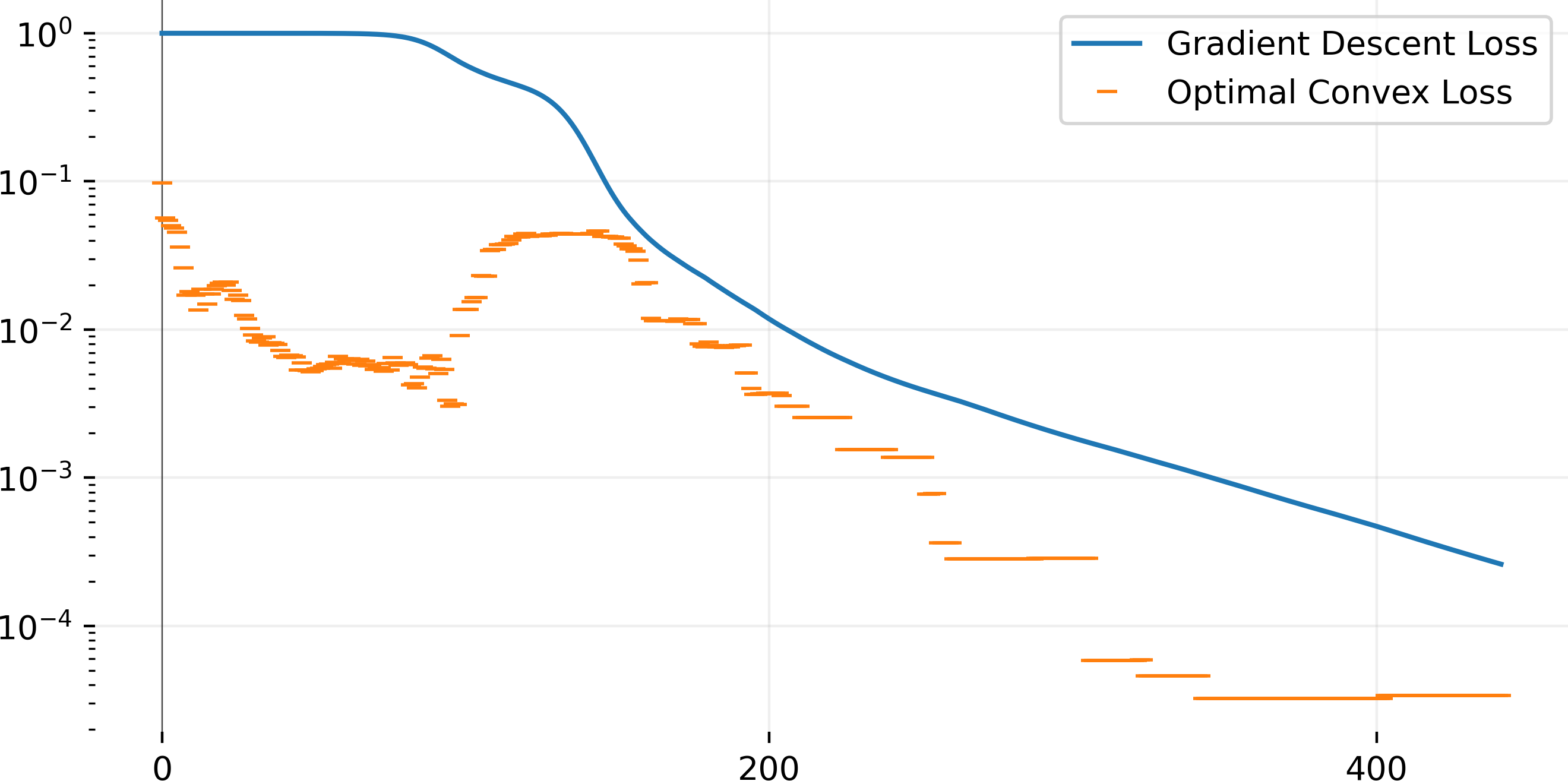
Training a 20-neuron network with gradient descent and using the same activation patterns to solve the convex equivalent. We plot for each step, the current loss of the non-convex network and the optimal loss of the convex problem. At initialization (first point on the graph), the non-convex loss is 1. We take the current activation pattern and build a convex problem and solve it, we find an optimal loss of $0.1$. In the next step, the non-convex loss decreases and the activation pattern has changed, thus we find a different optimal loss for the convex problem. The initial optimal loss of the convex is quickly beaten by gradient descent (at around step 175), this means that the activation patterns at step 0 were far from optimal. The convex loss at the start is quickly beaten by gradient descent, this means our initial choice of activation pattern was bad, and gradient descent continually improves them. We use cvxpy to define the problem and solve it using ECOS.
In general, we cannot predict which patterns will be used by the neurons found by GD, or which patterns are the best. Thus we cannot hope that the convex problem will give us an insight as it requires us to know the activation patterns.
In the next section, we focus on cases where the non-convex minima can be accurately described by convex problems.
On large initialization scale
The initialization scale of the network is the absolute size of the neurons’ parameters. To get a change in the scale, we can simply multiply every parameter by a scalar. The initial value of the neuron is a large topic in machine learning as it has a large influence on the quality of the local minimum. By default in popular libraries, He initialization
We say we are on a large scale when neurons do not move far from their initial value during descent. This typically happens when using large initial values for the parameters of each neuron.
The theory states that you can push the scale used high enough so that neurons will not change their activation patterns at all. If this is verified, the convex reformulation will describe exactly the minima that gradient descent will reach. However, it is not possible to observe this in practice as the loss becomes very small and the training process is too slow to carry on to the end. The NTK briefly mentioned in the introduction operates in this setting, using the fact that the network is very close to its linear approximation. On a similar note, reducing the step size for the first layer guarantee convergence
Illustration.
Using an animation, we plot every step of a gradient descent in the non-convex problem until the loss is small enough. As mentioned before, the training is too slow to continue until we reach a real local minimum described by the convex problem here. We plot the output of the network, which is the sum of all the neurons. We want to focus on the activation point of each neuron.
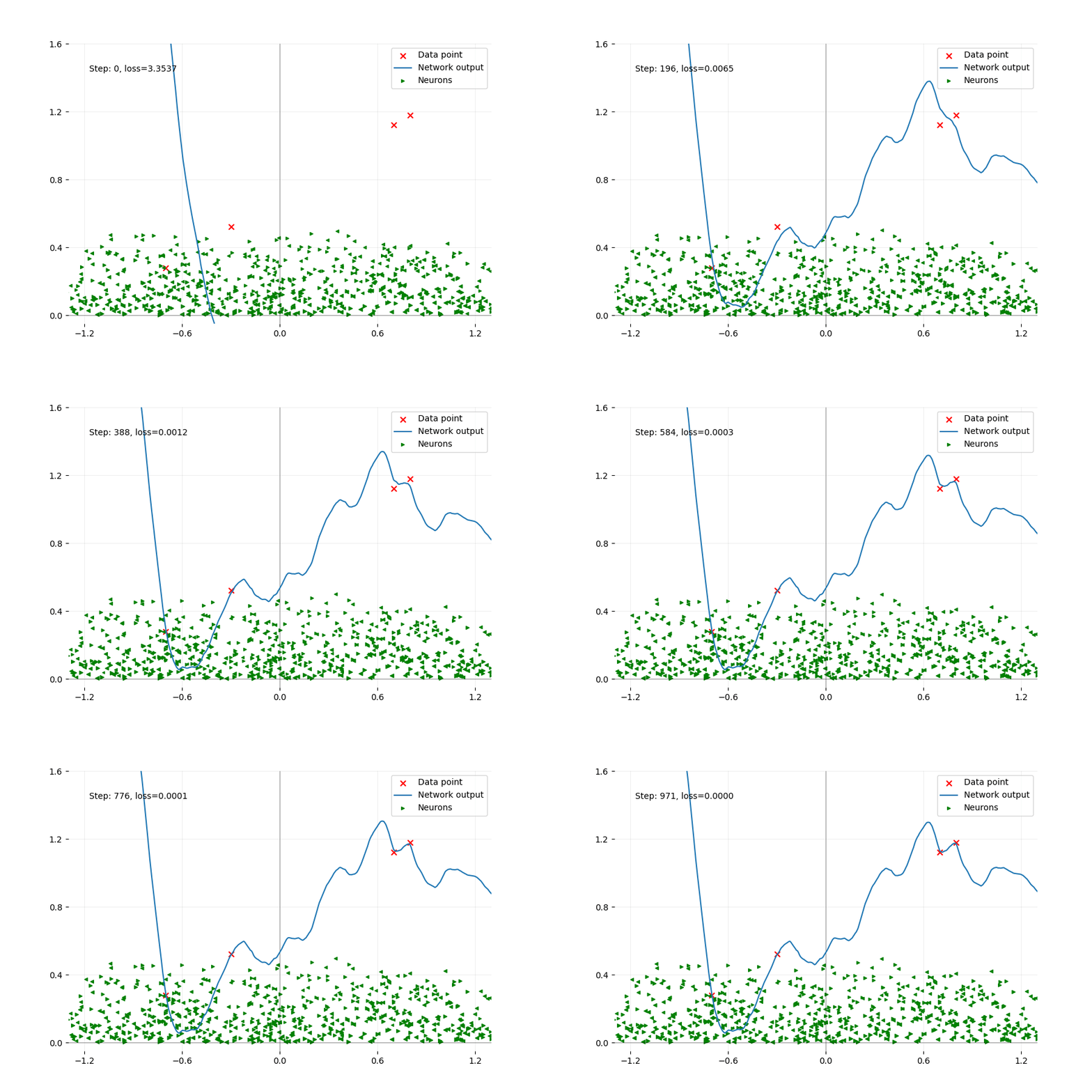
Training a network with 1000 neurons with big initial values using gradient descent. The output of the network is in blue, and the four data points (red crosses) represent linear data. Each green triangle represents one neuron with its activation point horizontally, and its norm vertically. The orientation of the triangle reveals which side the neuron will activate the data. At initialization, the repartition of the activation point is uniform. The movement of the activation point is minimal, only a few neurons will change their patterns, among the thousands.
Here, computing the convex optimal gives us a single neuron to fit the linear data. While the non-convex problem has converged to very low loss, their outputs are completely different.
A side effect of the large initialization is catastrophic overfitting i.e. there are very large variations between data points which will negatively impact test loss.
On very small initialization
At the other extreme, the small-scale setting effectively lets neurons align themselves before ever decreasing the loss. In theory, if you push the scale down enough, neurons will converge to a finite set of directions before trying to fit the objective.

Training a network with 1000 neurons with very small initial values using gradient descent. The output of the network is in blue, the four data points (red crosses) represent linear data. Each green triangle represents one neuron with its activation point horizontally, and its norm vertically. The orientation of the triangle reveals which side the neuron will activate the data. At initialization, the repartition of the activation point is uniform. However, as training progresses most neurons that activate toward the right converge to $-1.3$. Once the norm of the neuron at activating at $-1.3$ is large enough, the loss decreases and we quickly reach convergence.
Taking a look at the loss on the same problem, we can identify the two distinct regimes: alignment and fitting (then convergence).

Plot of the loss during gradient descent in the same setting as the animation above. In the first half only the directions of the neurons are changing (i.e. their activation patterns), and start fitting the four data points once their parameters are large enough.
If you take orthogonal data and a small scale, the behavior is very predictable
Unless mentioned otherwise, all experiments were run using full batch vanilla gradient descent. In experiments, it is clear that adding momentum or using the Adam optimizer is much easier to use on top of being faster to converge. However, the behavior is much less predictable.
Conclusion
The main takeaway is that the best network for a given dataset can be found exactly by solving a convex problem. Additionally, the convex problem can describe every local minimum found by gradient descent in the non-convex setting. However, finding the global optima is impossible in practice, and approximations are still costly in precision. While there is no evident link between feature learning in the non-convex and the convex reformulation, many settings allow for a direct equivalence and the whole convex toolkit for proofs.
The performance side of the convex reformulation will benefit from dedicated software as has been the case for gradient descent in deep networks. Only then will it offer a no-tuning alternative to costly stochastic gradient descent. In smaller settings, it already allows us to quickly find all the possible local minima that are so important in machine learning.
Despite advancements in understanding the optimization landscape of neural networks, a significant gap persists in reconciling theory with practical challenges, notably because of early stopping. In real-world scenarios, networks often cease learning before reaching a local minimum and this has a direct impact (in large-scale initialization) but there are limited results.
Acknowledgements
This work is partly funded by the ANR JCJC project ANR-21-CE23-0022-01.