Fairness in AI: two philosophies or just one?

The topic of fairness in AI has garnered more attention over the last year, recently with the arrival of the EU's AI Act. This goal of achieving fairness in AI is often done in one of two ways, namely through counterfactual fairness or through group fairness. These research strands originate from two vastly differing ideologies. However, with the use of causal graphs, it is possible to show that they are related and even that satisfying a fairness group measure means satisfying counterfactual fairness.

This blog post is based on the paper of Anthis and Veitch. The original paper is enriched with a wide overview of fairness concepts used in research and visuals aiding the readers in gaining a deeper understanding. The blog post aims to raise questions about the dichotomy between procedural and outcome fairness, that they perhaps should not be treated as separate research fields as is currently often the case.

Why fairness?

The spread of AI exposed some of the dark patterns that are present in society. Some well known examples are the COMPAS case which showed discrimination against black defendants and the Amazon hiring tool which showed a preference towards men compared to women. However, these AI system were most likely not the source of this disparate treatment. This behavior stems from the data that was used to train the system, thus this behavior comes from people who were behind the creation of that data.

Fairness in AI is a research strain which aims to remove the biases in the AI models that result in that disparate treatment. The goal of these models is that people are treated more fairly, perhaps even more than a human decision.

What is fairness?

The question of what is fair does not have a single answer. Even when stepping away from the computer science context, a universal definition, that can be used to determine if something is fair or not, cannot be found. The concept of fair is heavily influenced by a person, but also society’s biases. The fluidity of the notion therefore gives rise to multiple philosophies in what a fair AI system would be.

Figure 1: Some examples of the concepts used in the respective philosophies.

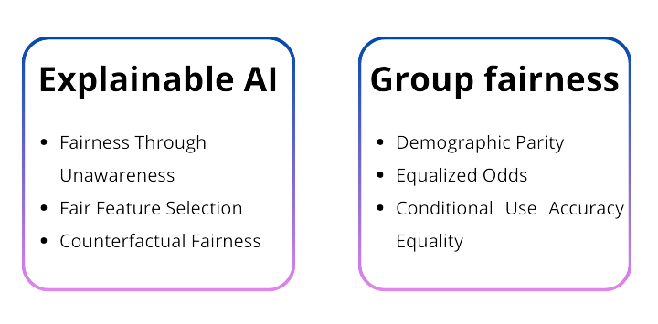
Two main philosophies can be found in research. The first one, often called explainable AI, aims to either create explainable models or to create explanations for the results obtained from a model. This can also be described as aiming for procedural fairness. The second philosophy is called group fairness. Group fairness focusses on outcome fairness. This means that the predictions from the AI system should have similar properties across groups that only differ in a certain personal attribute.

Explainable AI

The most famous example of explainable AI is fairness through unawareness. Fairness through unawareness means that no personal attributes are passed into the system, unless these are relevant for the prediction. The system does therefore not have access to the personal attributes, which means it cannot directly discriminate. Fairness through unawareness is often used as the basic model for fairness. However, the systems from both the COMPAS and Amazon example used fairness through unawareness and they still exhibited disparate treatment. The personal attributes that were removed from the data still had an influence on the dataset itself. For instance, a ZIP code can function as a proxy for race or someone’s gender influenced their writing style.

Figure 2: Examples of Fairness Through Unawareness (FTU) and fair feature selection on the Adult dataset.

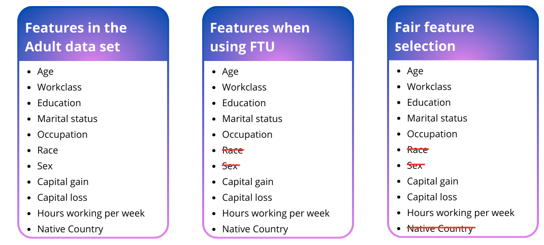
Related to fairness through unawareness is fair feature selection . Instead of removing the personal attributes, only features that are deemed appropriate remain in the dataset. It needs to be noted that one universal agreement for what are fair features to use is unlike due to the aforementioned biases of people and cultures. Oftentimes, there exists an overlap between the features removed in fairness through unawareness and fair feature selection as is evident in Figure 2.

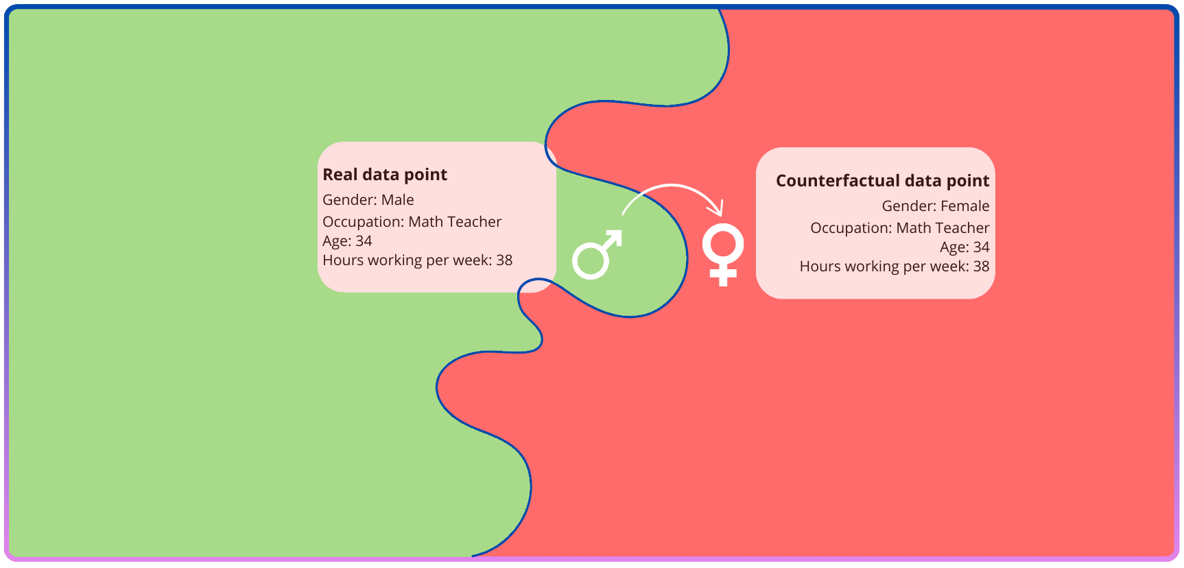
Counterfactual fairness is a currently popular type of explainable AI. Counterfactual fairness stems from systems that check for direct discrimination, meaning that simply changing a personal attribute would change a person’s prediction. An example of direct discrimination can be found in Figure 3, where changing the sex would result into a different prediction. From a legal standpoint it is clear that if a model would exhibit this behavior, it can be deemed unfair.

Figure 3: Example of direct discrimination where changing the personal attribute of sex changes the prediction a person would receive.

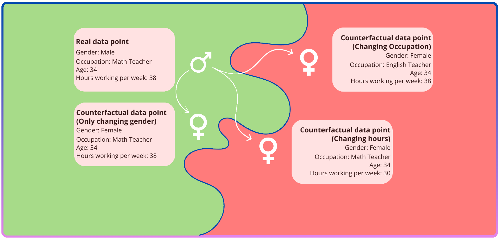
Models for counterfactual fairness change both the personal attributes of a person and other features are also adjusted according to a causal model related to the personal attributes. For example changing someone’s race might also require to change someone’s ZIP code or high school they went to. Figure 4 contains an example of creating counterfactuals. That system is unfair as some of the counterfactuals have a different prediction from the original. Satisfying counterfactual fairness can also be achieved through requiring independence between the personal attributes and the prediction itself. A more stringent constraint is to require that the prediction is independent on all proxy features in the dataset.

Figure 4: Imaginary examples of a system that would not satisfy counterfactual fairness. Changing features in accordance with the personal attributes and data distribution results in a different prediction.

Group Fairness

Group fairness is a different philosophy regarding fairness of an AI system. Instead of requiring the process of the system is fair, it requires the outcome of the model to be fair. This verdict of fairness is based on the equality of a chosen statistical measure between groups. People are divided into these groups based on their personal attributes. Three definitions are most commonly used for group fairness namely, demographic parity, equalized odds and conditional use accuracy equality.

Demographic parity requires that the selection rate is equal across groups. This means that an equal percentage of people from both groups receives a positive prediction. This definition is independent of the ground truth, which means that for example a perfect predictor could never satisfy demographic parity if the base rates differ between groups. Therefore, from the observation of the dataset it must seem that the prediction is independent of the personal attributes.

Figure 5: A representation of demographic parity. Two groups are distinguished one male, one female. The circled individuals are the ones to receive a positive prediction.

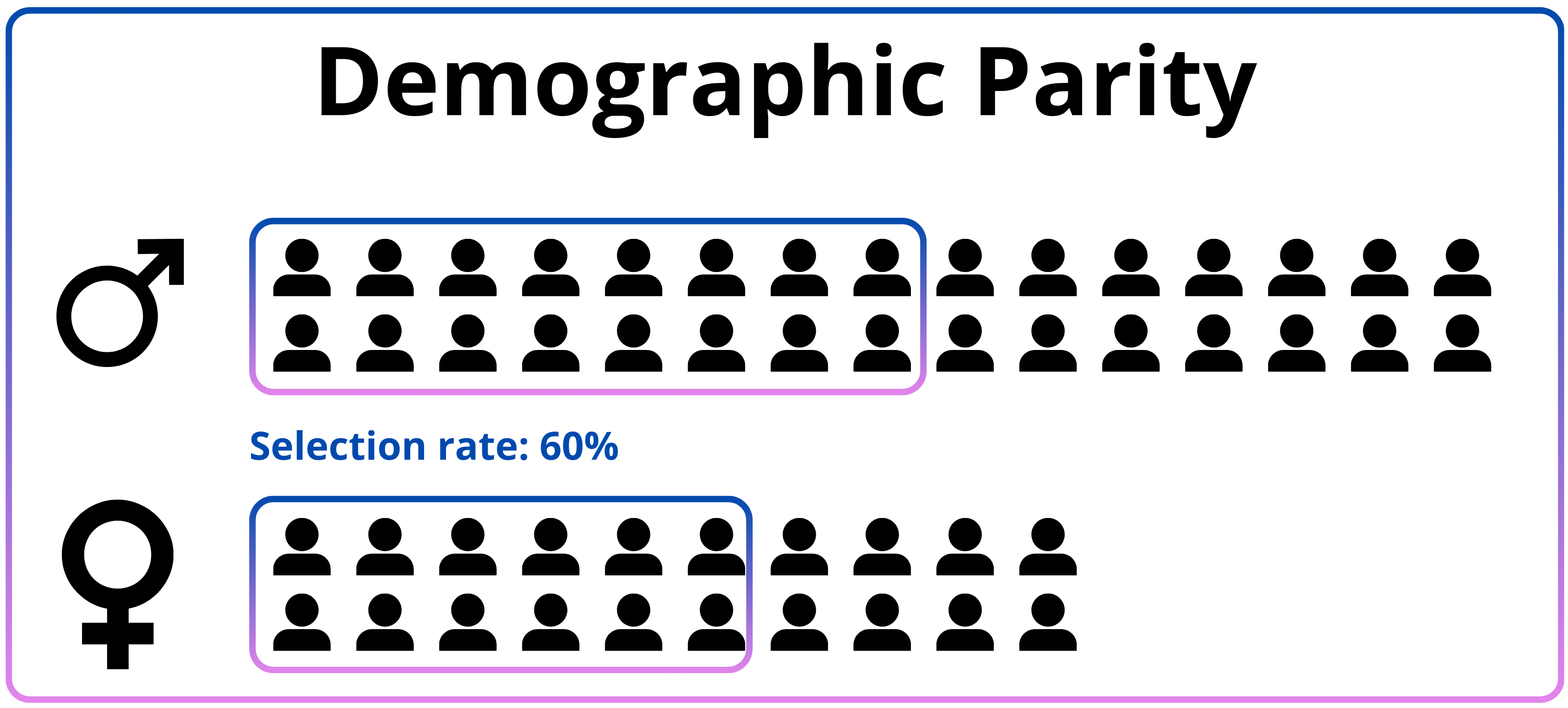
A second fairness measure used in group fairness in equalized odds. This fairness measure requires that both the true positive and true negative rates are equal across groups. This means that given the ground truth, there is an equal chance of giving a positive prediction irrespective of a person’s group. In other words equalized odds requires the prediction is independent of the personal attribute given the ground truth. Unlike demographic parity, equalized odds is dependent on the ground truth.

Figure 6: A representation of predictions which satisfy equalized odds. Two groups are distinguished one male, one female. The circled individuals are the ones to receive a positive prediction. The colors of the individuals indicates the ground truth of the samples. The male groups has a base rate of 0.8 and the female group a base rate of 0.6.

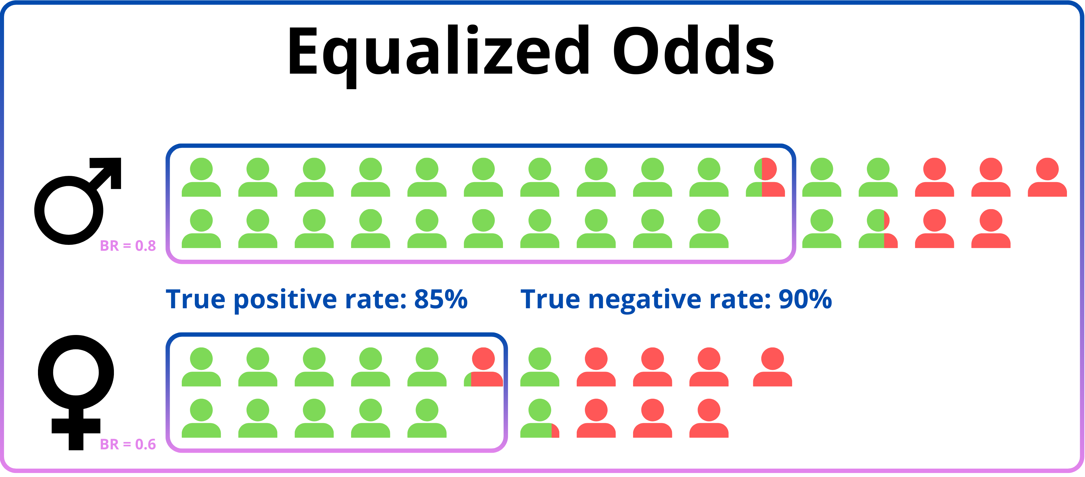
The final common fairness measure in group fairness is conditional use accuracy equality. In order to satisfy conditional use accuracy equality, the precision and false omission rate must be equal between groups. Similar to equalized odds, conditional use accuracy equality requires two statistical properties to be equal between groups, namely precision and false omission rate. Put differently, this requires that given the prediction there is an equal chance that this prediction is correct regardless of the group a person belongs to. Conditional use accuracy equality is therefore defined similarly to equalized odds; the roles of the prediction and ground truth are simply reversed. This equality also holds for the independent condition, conditional use accuracy equality requires that the ground truth is independent of the personal attribute if the prediction is known.

Figure 7: A representation of predictions which satisfy conditional use accuracy equality. Two groups are distinguished one male, one female. The circled individuals are the ones to receive a positive prediction. The colors of the individuals indicates the ground truth of the samples. The male groups has a base rate of 0.8 and the female group a base rate of 0.6.

Unifying these philosophies

The previous two sections discussed the different concepts used for explainable AI and group fairness. It is clear that they employ a different basis for their philosophy of fairness. However, when looking at these definitions, the concept of independence returns in both counterfactual fairness and the fairness measures used for group fairness. This property of requiring independence allows to unify these notions that they accomplish the same result. Table 1 provides an overview of the fairness measures and the respective independence they require.

In the following section \(Y\) symbolises the perceived label, \(D\) the prediction, \(A\) the personal attributes, \(S\) the selection of a sample in the dataset, \(X^{\bot}_A\) the data independent of the personal attributes, \(X^{\bot}_Y\) the data independent of the prediction and \(\tilde{Y}\) the real label.

Table 1: A summary of the independence requirement of the fairness notions discussed.

Name	Probability definition	Independence
Demographic parity	\(P(D=1\vert A=1) = P(D=1\vert A=0)\)	\(D \bot A\)
Equalized odds	\(P(D=1 \vert A=1, Y=y) = P(D=1 \vert A=0, Y=y)\)	\(D \bot A \vert Y\)
Conditional use accuracy equality	\(P(Y=1\vert A=1, d=y) = P(D=1 \vert A=0, D=y)\)	\(Y \bot A \vert D\)

Measurement error - Demographic parity

Figure 8: A directed acyclic graph showing the relation between the prediction and the data, in the situation of measurement error.

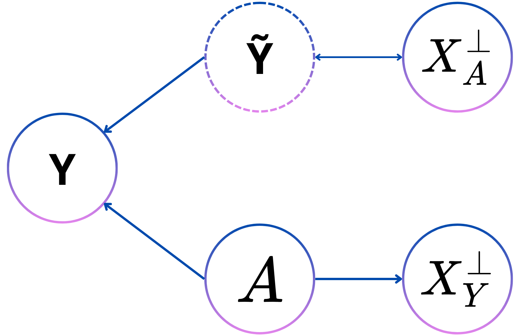
Measurement error is a first type of dependence that can be resolved in order to be counterfactually fair. Measurement errors means that there is some bias on the perceived ground truth in the dataset. For example in system that determines whether pulling a car over is justified or not (whether a crime was committed or not). More crimes can be uncovered if a full car search happens, however a car search is not always undertaken resulting in a bias of more positive samples for a population where a car search is more likely to happen. In this situation the label is whether or not a crime was detected, not wether a crime was committed. The imbalance car searches for a group with a certain personal attribute will then have an effect on the label. This influence of the personal attributes on the label, but not the ground truth is shown in Figure 6.

A second example of measurement error can be found in healthcare prediction. Predicting someone’s health is abstract as this is not quantifiable. A proxy for health is the costs related to the healthcare an individual receives. However, costs are not universal for each group in society. Certain groups can thus have lower costs while managing more health problem due to the care that they receive or perhaps not receive. This faulty proxy is another example of measurement errors.

This system is thus made counterfactually fair if the dependence between the personal attribute and the label is removed. The same independence that is requires to satisfy demographic parity.

Selection on label - Equalized odds

Figure 9: A directed acyclic graph showing the relation between the prediction and the data, in the situation of selection on label.

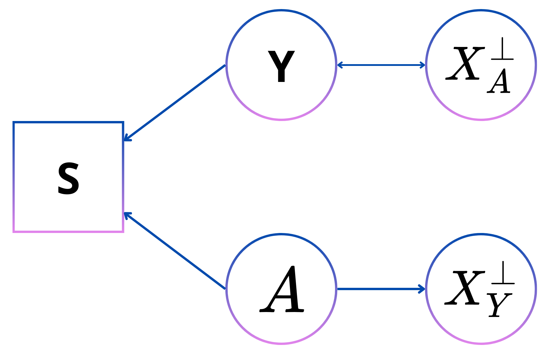
Selection on label is a type of bias that arises by that not only someone’s label affects their adoption in the dataset but also their personal attribute. A subtype of this type of bias is self-selection bias. This means that certain groups of the population are more represented in certain dataset due to that certain groups are more likely to interact with the data collection system. An example of this is in voluntary studies where certain groups are more likely to participate than others leading to a skewed dataset in favor of the participating group. A study around self-selection bias in nutrition trials also found that a person’s ground truth influences their participation in the trial (healthy eaters were more likely to apply for this trial).

The directed acyclic graph in Figure 7 shows how to decouple the label itself with the personal attribute by introducing the variable of the selection bias in S, which is an observed variable. \(A\) and \(X^{\bot}_A\) are only connected through a path that includes \(Y\) which means that given \(Y\), \(A\) and \(X^{\bot}_A\) are independent, which is the condition of equalized odds.

Selection on predictor - conditional use accuracy equality

Figure 10: A directed acyclic graph showing the relation between the prediction and the data, in the situation of selection on predictor.

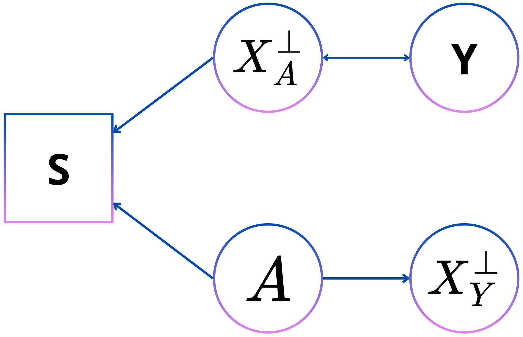
Selection on predictor is similar to selection on label, but instead of the label influencing the prediction is it the features themselves that influence the prediction together with the personal attributes. An example of this can be seen in the student population of engineering degrees. A relevant feature such as what a person studied in high school influence their choice to do engineering. However, there is a large discrepancy in the number of male versus female student who pursue engineering even though that difference does not exist in that degree when graduating high school. This shows that both relevant features, but also personal attributes influence their presence in a dataset about engineering students.

The acyclic graph in Figure 8 for selection on predictor is similar to that for selection on label. The features and label are simply reversed in this situation. This is also in accordance with the similarity seen between equalized odds and conditional use accuracy equality. Through \(X^{\bot}_A\), are \(A\) and \(Y\) connected, which means that if the prediction is known, which is captured in \(X^{\bot}_A\), then \(A\) and \(Y\) are independent, which is necessary to satisfy conditional use accuracy.

Confirmation with experiments

This relation between counterfactual fairness and group fairness is supported by experiments. These experiments were done on a synthetic version of the Adult dataset. A simulated protected class A was added where the incidence is balanced (50/50 odds of belonging to the protected class or not). If someone belonged to the protected class, then there is a causal effect of A on X: \(P(race=other) = 0.8\). This thus means that A will loosely relate to someone’s race being noted as “other”. This dataset serves as the target distribution for the biased datasets.

A counterfactually fair model is achieved by by taking the average prediction of an instance if it were part of the protected class and if it was not. Three biased datasets are created based on the directed acyclic graphs in Figures 8, 9, and 10. Table 2 shows that satisfying counterfactual fairness for a certain type of dataset will satisfy a corresponding fairness measure, confirming the theoretical results above.

Table 2: The results of applying counterfactual fairness to a model with its performance on different fairness measures.

	Demographic parity difference	Equalized odds difference	Conditional use accuracy equality
Measurement Error	-0.0005	0.0906	-0.8158
Selection on Label	0.1321	-0.0021	0.2225
Selection on Predictors	0.1428	0.0789	0.0040

What can we take away?

Procedural and outcome fairness have tended to coexist in research. They are each their own field with their philosophy with the common goal of creating fairer AI systems. The strengths of techniques like counterfactual fairness lie in their explainability and thus allow for an easier determination of whether they are fair or not. The group fairness techniques know many implementations and have been proven to be powerful. However, they are not very interpretable. In order to determine what is fair a first abstraction must be made into converting the meaning of fairness into a mathematical fairness measure. The determination of whether the system is fair is thus dependent on the interpretation of the fairness measure and the quality of the dataset. If the dataset is not representative then there is no guarantee that the system will have a fair outcome.

This relation between the procedural fairness and outcome fairness opens certain research possibilities, perhaps allowing for the strength of the outcome fairness techniques to be combined with the interpretability of the procedural fairness concepts. A future research possibility is to investigate if the techniques to satisfy fairness measure also satisfy some explainability notions or what adjustments would be needed.