Elaborating on the Value of Flow Matching for Density Estimation

The transfer of matching-based training from Diffusion Models to Normalizing Flows allows to fit expressive continuous normalizing flows efficiently and therefore enables their usage for different kinds of density estimation tasks. One particularly interesting task is Simulation-Based Inference, where Flow Matching enabled several improvements. The post shall focus on the discussion of Flow Matching for Continuous Normalizing Flows. To highlight the relevance and the practicality of the method, their use and advantages for Simulation-Based Inference is elaborated.

Motivation

Normalizing Flows (NF) enable the construction of complex probability distributions by transforming a simple, known distribution into a more complex one. They do so by leveraging the change of variables formula, defining a bijection from the simple distribution to the complex one.

For most of the time, flows were based on chaining several differentiable and invertible transformations. However, these diffeomorphic transformations limit the flows in their complexity as such have to be simple. Furthermore, this leads to trade-off sampling speed and evaluation performance . Their continuous counterpart, Continuous Normalizing Flows (CNFs) have been held back by limitations in their Simulation-Based maximum likelihood training . By utilizing Flow Matching, this limitation has been overcome and CNFs have been shown to be a powerful tool for density estimation.

In the following sections, CNFs and Flow Matching are explained. Following the explanation, the empirical results of Flow Matching are presented. Finally, the application of Flow Matching in Simulation-Based Inference is discussed, which shall highlight their wide applicability and consistent improvement.

Continuous Normalizing Flows

Continuous normalizing flows are among the first applications of neural ordinary differential equations (ODEs) . Instead of the traditional layers of neural networks, the flow is defined by a vector field that is integrated over time.

\[\frac{d}{dt} x(t) = f_{\theta}(x(t), t)\]

The vector field is typically parameterized by a neural network. While traditional layer based flow architectures need to impose special architectural restrictions to ensure invertibility, CNFs are invertible as long as the uniqueness of the solution of the ODE is guaranteed. This is for instance the case if the vector field is Lipschitz continuous in \(x\) and continuous in \(t\). Many common neural network architectures satisfy these conditions. Hence, the above equation defines a diffeomorphism \(\phi_t(x_0) = x_0 + \int_0^t f_{\theta}(x(t), t)\) under the discussed assumption. The change of variables formula can be applied to compute the density of a distribution that is transformed by \(\phi_t\).

As usual, a CNF is trained to transform a simple base distribution \(p_B\), usually a standard normal distribution, into a complex data distribution \(p_D\). For each point in time \(t\in[0,1]\) the time-dependent vector field defines a distribution \(p_t\) (probability path) and the goal is to find a vector field \(f_\theta\) such that \(p_1=p_D\). This is usually achieved by maximum likelihood training, i.e. by minimizing the negative log-likelihood of the data under the flow.

While CNFs are very flexible, they are also computationally expensive to train naively with maximum likelihood since the flow has to be integrated over time for each sample. This is especially problematic for large datasets which are needed for the precise estimation of complex high-dimensional distributions.

Flow Matching

The authors of propose a new method for training CNFs, which avoids the need for simulation. The key idea is to regress the vector field directly from an implicit definition of a target vector field that defines a probability path \(p_t(x)\) with \(p_0=p_{B}\) and \(p_1=p_{D}\). Moreover, the authors propose a loss function that directly regresses the time dependent vector field against the conditional vector fields with respect to single samples.

Unconditional ImageNet-128 samples of a CNF trained using Flow Matching with Optimal Transport probability paths. Figure obtained from .

Assuming that the target vector field is known, the authors propose a loss function that directly regresses the time dependent vector field:

\[L_{\textrm{FM}}(\omega) = \mathbb{E}_{t, p_t(x)}(|f_{\omega}(x, t) - u_t(x)|^2),\]

where \(u_t\) is a vector field that generates \(p_t\) and the expectation with respect to \(t\) is over a uniform distribution. Unfortunately, the loss function is not directly applicable because we do not know how to define the target vector field. However, it turns out that one can define appropriate conditional target vector fields when conditioning on the outcome \(x_1\):

\[p_t(x) = \int p_t(x|x_1)p_{D}(x_1)d x_1.\]

Using this fact, the conditional flow matching loss can be defined, obtaining equivalent gradients as the flow matching loss.

\[L_{\textrm{CFM}}(\omega) = \mathbb{E}_{t, p_t(x|x_1), p_D(x_1)}(|f_{\omega}(x, t) - u_t(x|x_1)|^2).\]

Finally, one can easily obtain an unbiased estimate for this loss if samples from \(p_D\) are available, \(p_t(x|x_1)\) can be efficiently sampled, and \(u_t(x|x_1)\) can be computed efficiently. We discuss these points in the following.

Gaussian Conditional Probability Paths

The vector field that defines a probability path is usually not unique. This is often due to invariance properties of the distribution, e.g. rotational invariance. The authors focus on the simplest possible vector fields to avoid unnecessary computations. They choose to define conditional probability paths that maintain the shape of a Gaussian throughout the entire process. Hence, the conditional probability paths can be described by a variable transformation \(\phi_t(x \mid x_1) = \sigma_t(x_1)x + \mu_t(x_1)\). The time-dependent functions \(\sigma_t\) and \(\mu_t\) are chosen such that \(\sigma_0(x_1) = 1\) and \(\sigma_1 = \sigma_\text{min}\) (chosen sufficiently small), as well as \(\mu_0(x_1) = 0\) and \(\mu_1(x_1)=x_1\). The corresponding probability path can be written as

\[p_t(x|x_1) = \mathcal{N}(x; \mu_t(x_1), \sigma_t(x_1)^2 I).\]

In order to train a CNF, it is necessary to derive the corresponding conditional vector field. An important contribution of the authors is therefore the derivation of a general formula for the conditional vector field \(u_t(x|x_1)\) for a given conditional probability path \(p_t(x|x_1)\) in terms of \(\sigma_t\) and \(\mu_t\):

\[u_t(x\mid x_1) = \frac{\sigma_t'(x_1)}{\sigma_t(x_1)}(x-\mu_t(x_1)) - \mu_t'(x_1),\]

where \(\psi_t'\) denotes the derivative with respect to time \(t\).

Compared to the diffusion path’s conditional score function, the OT path’s conditional vector field has constant direction in time and is arguably simpler to fit with a parametric model. Note the blue color denotes larger magnitude while red color denotes smaller magnitude. Figure obtained from .

They show that it is possible to recover certain diffusion training objectives with this choice of conditional probability paths, e.g. the variance preserving diffusion path with noise scaling function \(\beta\) is given by:

\[\begin{align*} \phi_t(x \mid x_1) &= (1-\alpha_{1-t}^2)x + \alpha_{1-t}x_1 \\\ \alpha_{t} &= \exp\left(-\frac{1}{2}\int_0^t \beta(s) ds\right) \end{align*}\]

Additionally, they propose a novel conditional probability path based on optimal transport, which linearly interpolates between the base and the conditional target distribution.

\[\phi_t(x \mid x_1) = (1-(1-\sigma_{\text{min}})t)x + tx_1\]

The authors argue that this choice leads to more natural vector fields, faster convergence and better results.

Empirical Results

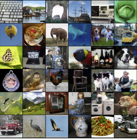
The authors investigate the utility of Flow Matching in the context of image datasets, employing CIFAR-10 and ImageNet at different resolutions. Ablation studies are conducted to evaluate the impact of choosing between standard variance-preserving diffusion paths and optimal transport (OT) paths in Flow Matching. The authors explore how directly parameterizing the generating vector field and incorporating the Flow Matching objective enhances sample generation.

Likelihood (BPD), quality of generated samples (FID), and evaluation time (NFE) for the same model trained with different methods. Figure from .

The findings are presented through a comprehensive evaluation using various metrics such as negative log-likelihood (NLL), Frechet Inception Distance (FID), and the number of function evaluations (NFE). Flow Matching with OT paths consistently outperforms other methods across different resolutions.

Flow Matching, especially when using OT paths, allows us to use fewer evaluations for sampling while retaining similar numerical error (left) and sample quality (right). Results are shown for models trained on ImageNet 32×32, and numerical errors are for the midpoint scheme. Figure from .

The study also delves into the efficiency aspects of Flow Matching, showcasing faster convergence during training and improved sampling efficiency, particularly with OT paths.

Sample paths from the same initial noise with models trained on ImageNet 64×64. The OT path reduces noise roughly linearly, while diffusion paths visibly remove noise only towards the end of the path. Note also the differences between the generated images. Figure from .

Image super-resolution on the ImageNet validation set. Figure from .

Additionally, conditional image generation and super-resolution experiments demonstrate the versatility of Flow Matching, achieving competitive performance in comparison to state-of-the-art models. The results suggest that Flow Matching presents a promising approach for generative modeling with notable advantages in terms of model efficiency and sample quality.

Application of Flow Matching in Simulation-Based Inference

A very specifically interesting application of density estimation, i.e. Normalizing Flows, is in Simulation-Based Inference (SBI). In SBI, Normalizing Flows are used to estimate the posterior distribution of model parameters given some observations. An important factor here are the sample efficiency, scalability, and expressivity of the density model. Especially for the later two, Flow Matching has shown to the yield an improvement. This is due to the efficient transport between source and target density and the flexibility due the more complex transformations allowed by continuous normalizing flows. To start out, a brief introduction to SBI shall be given as not many might be familiar with this topic.

Primer on Simulation-Based Inference

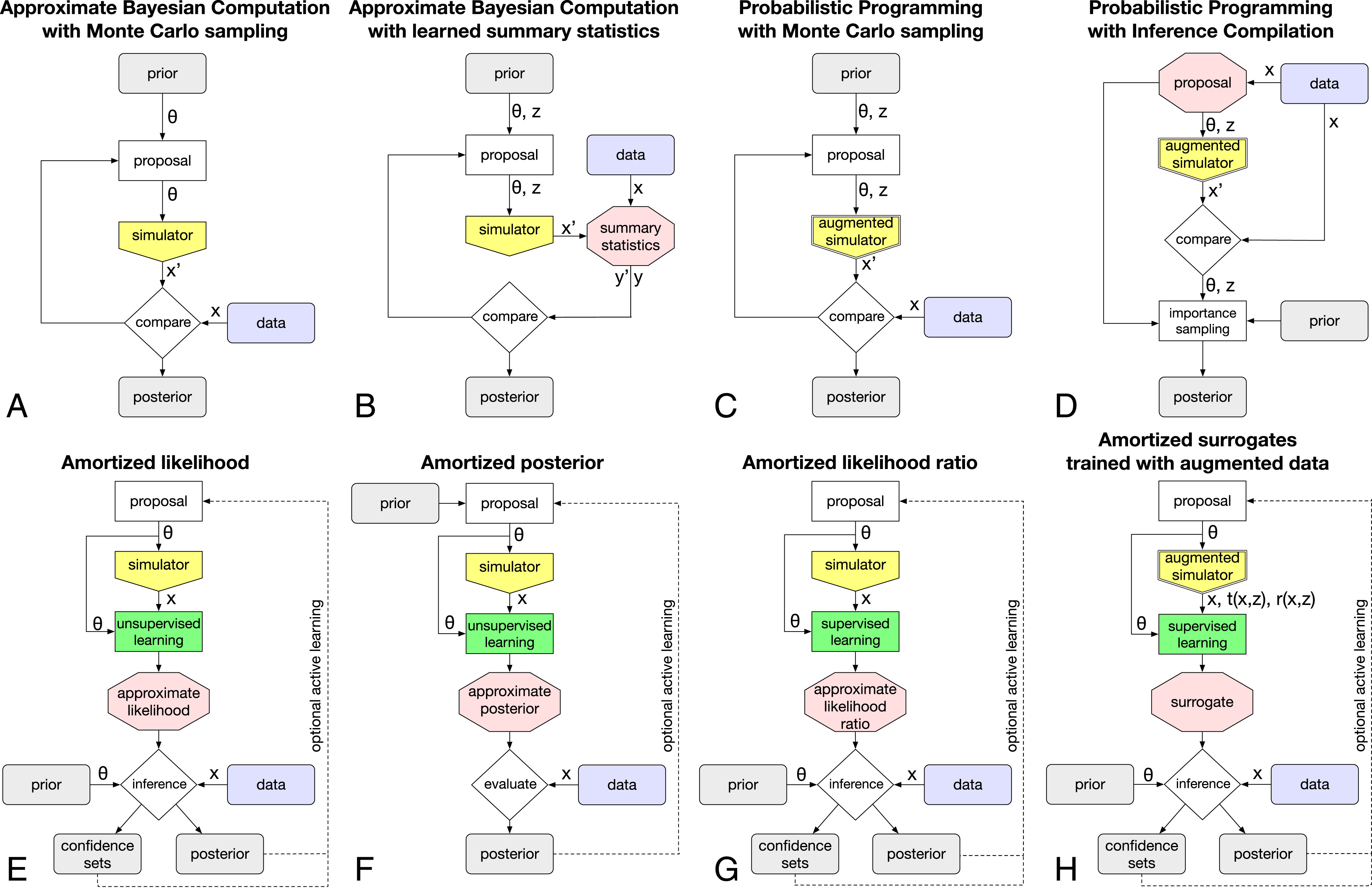
In many practical scenarios, the likelihood function of a model is intractable and cannot be described analytically. This might be the case for where the forward model is a complex or proprietary simulation, or if it is a physical experiment . In order to still be able to perform Bayesian inference, one can resort to a class of methods called Likelihood-free Inference. One possible but popular method in this class is SBI. The core idea is to use a prior in combination with the simulator to obtain samples from the joint distribution of the parameters and the data. Based on these samples, the posterior can either be learned directly or the likelihood can be approximated . Depending on the exact method chosen, the approximated posterior is either amortized, i.e. does not require refitting when conditioned on different data, or non-amortized.

The figure depicts the schematic flow of information for different kinds of Likelihood-free methods. Modern methods in SBI are depicted in the bottom row where the likelihood is approximated in subfigure E, the posterior is approximated in subfigure F, and the likelihood-ratio in subfigure G. Figure from .

In order to formalize the method, let \(\theta \sim \pi(\theta)\) denote the parameters to a system and its respective prior distribution. The system under evaluation and the respective observations obtained are denoted by \(x = \mathcal{M}(\theta)\). To sample from the joint distribution \(p(\theta, x)\), the dedicated parameter \(\theta_i\) is sampled from the prior and the observation is obtained by evaluating the forward model on that parameter \(x_i = \mathcal{M}(\theta_i)\). According to this approach, a dataset of samples from the joint distribution can be generated \(\mathcal{X} = \{ (\theta, \mathbf{x})_i \}^N_{i=1}\). A density estimator is then fitted on the provided dataset in order to estimate the desired distribution, e.g. directly the posterior \(q_{\omega}(\theta \mid x) \approx p(\theta \mid x)\).

The interested reader shall be directed to and especially for a more rigorous introduction to SBI. In order to compare the performances of the different approaches to SBI and their performance with respect to certain tasks, an excellent overview is provided in . For the sake of this post, a more abstract understanding is enough.

Flow Matching for Simulation-Based Inference

The approach using the Flow Matching formulation to fit the density network is presented by Dax et al. . In the setting described by the authors and the before mentioned SBI context, the goal is to approximate a posterior distribution of over model parameters given observations \(p(\theta \vert x)\). To learn the posterior, the Flow Matching loss is adapted to the following:

\[\mathcal{L}_{FMPE} = \mathbb{E}_{t \sim p(t),\theta_1 \sim p(\theta), x \sim p(x \vert \theta_1),\theta_t \sim p_t(\theta_t \mid \theta_1)} \Vert f_{\omega,x}(\theta_t, t) - u_t(\theta_t \mid \theta_1) \Vert^2\]

The important details to note here are the adaptations to minimize the loss w.r.t. samples drawn from the joint distribution, as it is described in the general section to SBI. To do so, the expectation is adapted to be w.r.t. \(\theta_1 \sim p(\theta), x \sim p(x \vert \theta_1)\), which yield the desired samples.

Another adaption by the authors is to exchange the uniform distribution over the time with a general distribution \(t \sim p(t)\). The effects of this substitution won’t be focus deeper. However, adapting the distribution makes intuitive sense as the training gets harder close to the target distribution. Therefore, focussing on time steps \(t\) closer to one is beneficial, as the authors have also found in their empirical studies.

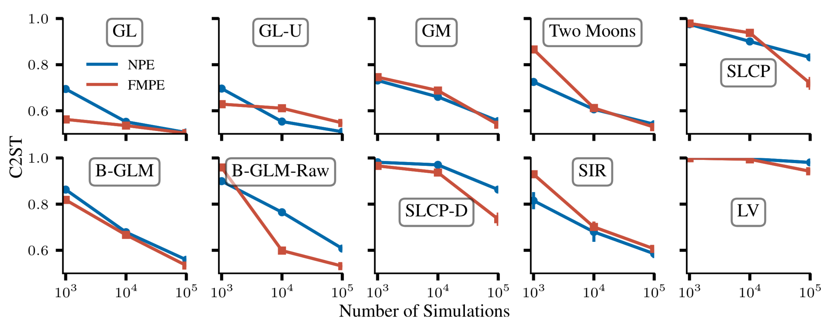
In order to provide a general comparison of the Flow Matching-based SBI approach, the CFM model is tested on the SBI benchmarking tasks . The results show either equal or better performance, underscoring the approaches ability and applicability to SBI.

The figure depicts the results of the CFM model on the SBI benchmarking tasks, as carried out by the authors of . Comparing the results to such obtained by neural posterior estimation with a normalizing flow shows comparable performance on most tasks while outperforming on some.

Besides the general benchmarks, the authors use their proposed technique to estimate the posterior distribution of gravitational wave parameters \(p(\theta \mid x)\) where \(\theta \in \mathbb{R}^{15}, x \in \mathbb{R}^{15744}\). In order to reduce the problem’s dimensionality and increase the information density, the observations are compressed to \(128\) dimensions using an embedding network.

Following the preprocessing of the data, three density estimators are fitted and compared to each other. The first method uses a neural spline flow, which has proven itself on these kinds of problems. It is compared to a neural posterior estimation using the Flow Matching approach described here. Finally, a neural posterior estimator leveraging physical symmetries is used to estimate the targeted posterior. All were trained on a simulation budget of \(5 \cdot 10^6\) samples for a total of 400 epochs.

In order to evaluate the models’ performances, the obtained posteriors were compared w.r.t. their 50% credible regions as well as Jensen-Shannon divergence between the inferred posterior and reference results. The results shown below support the advantages found in the benchmarking tasks. The Flow Matching-based shows a good performance for all shown parameters and has a clear advantage over the classical NPE approach.

The figure shows the single performances of a classic NPE approach using neural spline flows, the proposed Flow Matching approach, and a physics-focussed NPE approach. The results are shown for the 50% credible regions on the left, as well as the Jensen-Shannon divergence between the inferred posterior and reference results on the right. The Flow Matching-based approach shows a good performance for all investigated parameters and has a clear advantage over the classical NPE approach. In the pair plot on the left, the choice was made to only show the four parameters for which the classical NPE method performs the worst. While the Flow Matching approach could perform worse on other dimensions, this is not the case as shown on the right. Figure from .

Whilst the examples are interesting themselves, their evaluation has shown the applicability, scalability, and flexibility of Flow Matching for density estimation. These performance improvements in different areas have motivated the discussion of Flow Matching in the first place and hopefully become clear now.

A Personal Note

Whilst this is a blog post, we’d like to use this last part to express our personal thoughts on this topic. SBI is a powerful method, enabling Bayesian Inference where it would not be possibleIt might be more fitting to say that Bayesian Inference is not practically feasible in many scenarios as, in theory, it might still be possible by sampling. However, this is essentially not possible where single evaluations of the forward model are expensive or further evaluations are simply not available, as shown in the example. otherwise. Due to the natural problem setting of SBI, where problems are high-dimensional, observations are scarce, and distribution complex, density estimators capable to counter these are required. In the past, Normalizing Flows have proven themselves to meet these challenges, whilst not resolving them completely. CNFs, due to their higher flexibility, have been a desired method to put to test whether they could even improve on these but were limited in the inability to train the efficiently.

Formulating the Flow Matching variant of CNFs has allowed their application to complex density estimation tasks, as for example in SBI, and they’ve shown to yield the expected improvements – on standard SBI benchmarking tasks as well a very high dimensional task from the field of astrophysics. Furthermore, the generalization of CFM even broadens their applicability. It will be very interesting to see what possibilities are opened by this exact formulation and, in addition, what further improvements can be obtained by transferring techniques from the Diffusion Models to Normalizing Flows.