Double Descent Demystified
Identifying, Interpreting & Ablating the Sources of a Deep Learning Puzzle
Introduction
Machine learning models, while incredibly powerful, can sometimes act unpredictably. One of the most intriguing behaviors is when the test loss suddenly diverges at the interpolation threshold, a phenomenon distinctly observed in double descent
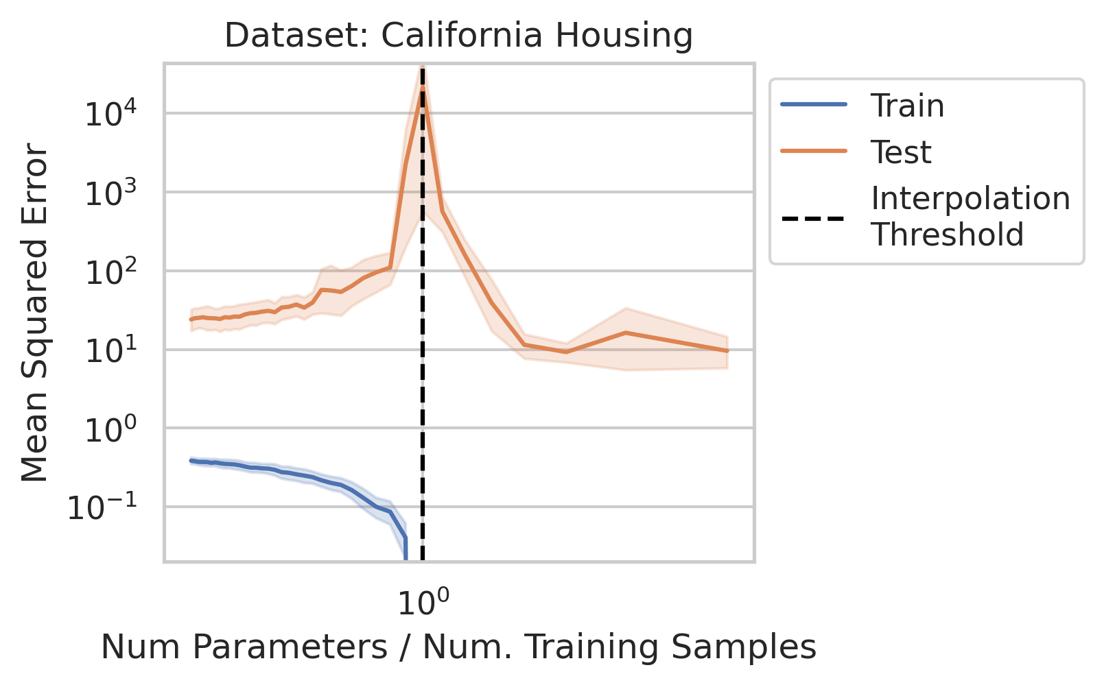
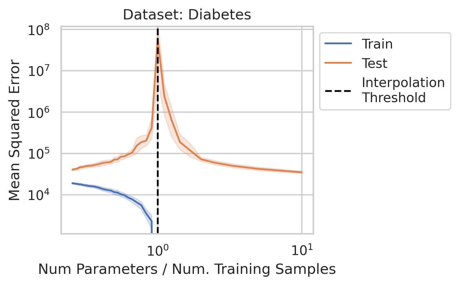

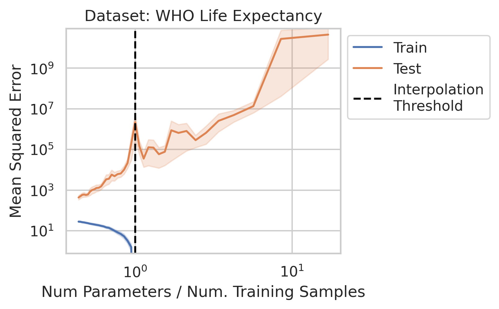
While significant theoretical work has been done to comprehend why double descent occurs, it can be difficult for a newcomer to gain a general understanding of why the test loss behaves in this manner, and under what conditions one should expect similar misbehavior. In this blog post, when we say double descent, we mean the divergence at the interpolation threshold, and not whether overparameterized models generalize (or fail to generalize).
In this work, we intuitively and quantitatively explain why the test loss diverges at the interpolation threshold, with as much generality as possible and with as simple of mathematical machinery as possible, but also without sacrificing rigor. To accomplish this, we focus on the simplest supervised model - ordinary linear regression - using the most basic linear algebra primitive: the singular value decomposition. We identify three distinct interpretable factors which, when collectively present, trigger the divergence. Through practical experiments on real data sets, we confirm that both model’s test losses diverge at the interpolation threshold, and this divergence vanishes when even one of the three factors is removed. We complement our understanding by offering a geometric picture that reveals linear models perform representation learning when overparameterized, and conclude by shedding light on recent results in nonlinear models concerning superposition.
Double Descent in Ordinary Linear Regression
Empirical Evidence of Double Descent in Ordinary Linear Regression
Before studying ordinary linear regression mathematically, does our claim that it exhibits double descent hold empirically? We show that it indeed does, using one synthetic and three real datasets: World Health Organization Life Expectancy
Notation and Terminology
Consider a regression dataset of $N$ training data with features $\vec{x}_n \in \mathbb{R}^D$ and targets $y_n \in \mathbb{R}$. We sometimes use matrix-vector notation to refer to the training data:
\[X \in \mathbb{R}^{N \times D} \quad , \quad Y \in \mathbb{R}^{N \times 1}.\]In ordinary linear regression, we want to learn parameters $\hat{\vec{\beta}} \in \mathbb{R}^{D}$ such that:
\[\vec{x}_n \cdot \hat{\vec{\beta}} \approx y_n.\]We will study three key parameters:
- The number of model parameters $P$
- The number of training data $N$
- The dimensionality of the data $D$
We say that a model is overparameterized if $N < P$ and underparameterized if $N > P$. The interpolation threshold refers to $N=P$, because when $N\leq P$, the model can perfectly interpolate the training points. Recall that in ordinary linear regression, the number of parameters $P$ equals the dimension $D$ of the covariates. Consequently, rather than thinking about changing the number of parameters $P$, we’ll instead think about changing the number of data points $N$.
Mathematical Analysis of Ordinary Linear Regression
To understand under what conditions and why double descent occurs at the interpolation threshold in linear regression, we’ll study the two parameterization regimes. If the regression is underparameterized, we estimate the linear relationship between covariates $\vec{x}_n$ and target $y_n$ by solving the least-squares minimization problem:
\[\begin{align*} \hat{\vec{\beta}}_{under} \, &:= \, \arg \min_{\vec{\beta}} \frac{1}{N} \sum_n ||\vec{x}_n \cdot \vec{\beta} - y_n||_2^2\\ \, &:= \, \arg \min_{\vec{\beta}} ||X \vec{\beta} - Y ||_2^2. \end{align*}\]The solution is the ordinary least squares estimator based on the second moment matrix $X^T X$:
\[\hat{\vec{\beta}}_{under} = (X^T X)^{-1} X^T Y.\]If the model is overparameterized, the optimization problem is ill-posed since we have fewer constraints than parameters. Consequently, we choose a different (constrained) optimization problem that asks for the minimum norm parameters that still perfectly interpolate the training data:
\[\begin{align*} \hat{\vec{\beta}}_{over} \, &:= \, \arg \min_{\vec{\beta}} ||\vec{\beta}||_2^2\\ \text{s.t.} \quad \quad \forall \, n \in &\{1, ..., N\}, \quad \vec{x}_n \cdot \vec{\beta} = y_n. \end{align*}\]We choose this optimization problem because it is the one gradient descent implicitly minimizes. The solution to this optimization problem uses the Gram matrix $X X^T \in \mathbb{R}^{N \times N}$:
\[\hat{\vec{\beta}}_{over} = X^T (X X^T)^{-1} Y.\]One way to see why the Gram matrix appears is via constrained optimization: define the Lagrangian $\mathcal{L}(\vec{\beta}, \vec{\lambda}) \, := \, \frac{1}{2}||\vec{\beta}||_2^2 + \vec{\lambda}^T (Y - X \vec{\beta})$ with Lagrange multipliers $\vec{\lambda} \in \mathbb{R}^N$, then differentiate with respect to the parameters and Lagrange multipliers to obtain the overparameterized solution.
After being fit, for test point $\vec{x}_{test}$, the model will make the following predictions:
\[\hat{y}_{test, under} = \vec{x}_{test} \cdot \hat{\vec{\beta}}_{under} = \vec{x}_{test} \cdot (X^T X)^{-1} X^T Y\] \[\hat{y}_{test, over} = \vec{x}_{test} \cdot \hat{\vec{\beta}}_{over} = \vec{x}_{test} \cdot X^T (X X^T)^{-1} Y.\]Hidden in the above equations is an interaction between three quantities that can, when all grow extreme, create a divergence in the test loss!
To reveal the three quantities, we’ll rewrite the regression targets by introducing a slightly more detailed notation. Unknown to us, there are some ideal linear parameters $\vec{\beta}^* \in \mathbb{R}^P = \mathbb{R}^D$ that truly minimize the test mean squared error. We can write any regression target as the inner product of the data $\vec{x}_n$ and the ideal parameters $\vec{\beta}^*$, plus an additional error term $e_n$ that is an “uncapturable” residual from the “viewpoint” of the model class
\[y_n = \vec{x}_n \cdot \vec{\beta}^* + e_n.\]In matrix-vector form, we will equivalently write:
\[Y = X \vec{\beta}^* + E,\]with $E \in \mathbb{R}^{N \times 1}$. To be clear, we are not imposing assumptions. Rather, we are introducing notation to express that there are (unknown) ideal linear parameters, and possibly non-zero errors $E$ that even the ideal model might be unable to capture; these errors $E$ could be random noise or could be fully deterministic patterns that this particular model class cannot capture. Using this new notation, we rewrite the model’s predictions to show how the test datum’s features $\vec{x}_{test}$, training data’s features $X$ and training data’s regression targets $Y$ interact.
Let $y_{test}^* := \vec{x}_{test} \cdot \vec{\beta}^*$. In the underparameterized regime:
\[\begin{align*} \hat{y}_{test,under} &= \vec{x}_{test} \cdot \hat{\vec{\beta}}_{under}\\ &=\vec{x}_{test} \cdot (X^T X)^{-1} X^T Y\\ &=\vec{x}_{test} \cdot (X^T X)^{-1} X^T (X \vec{\beta}^* + E)\\ &=\vec{x}_{test} \cdot \vec{\beta}^* + \, \vec{x}_{test} \cdot (X^T X)^{-1} X^T E\\ \hat{y}_{test,under} - y_{test}^* &= \vec{x}_{test} \cdot (X^T X)^{-1} X^T E. \end{align*}\]This equation is important, but opaque. To extract the intuition, replace $X$ with its singular value decomposition $X = U S V^T$. Let $R \, := \, \text{rank}(X)$ and let $\sigma_1 > \sigma_2 > … > \sigma_R > 0$ be $X$’s (non-zero) singular values. Let $S^+$ denote the Moore-Penrose inverse; in this context, this means that if a singular value $\sigma_r$ is non-zero, then in $S^+$, it becomes its reciprocal $1/\sigma_r$, but if the singular value is zero, then in $S^+$, it remains $0$. We can decompose the underparameterized prediction error along the orthogonal singular modes:
\[\begin{align*} \hat{y}_{test, under} - y_{test}^* &= \vec{x}_{test} \cdot V S^{+} U^T E\\ &= \sum_{r=1}^R \frac{1}{\sigma_r} (\vec{x}_{test} \cdot \vec{v}_r) (\vec{u}_r \cdot E). \end{align*}\]This equation will be critical! The same term will appear in the overparameterized regime (plus one additional term):
\[\begin{align*} \hat{y}_{test,over} &= \vec{x}_{test} \cdot \hat{\vec{\beta}}_{over}\\ &= \vec{x}_{test} \cdot X^T (X X^T)^{-1} Y\\ &= \vec{x}_{test} \cdot X^T (X X^T)^{-1} (X \beta^* + E)\\ \hat{y}_{test,over} - y_{test}^* &= \vec{x}_{test} \cdot (X^T (X X^T)^{-1} X - I_D) \beta^* \\ &\quad\quad + \quad \vec{x}_{test} \cdot X^T (X X^T)^{-1} E\\ &= \vec{x}_{test} \cdot (X^T (X X^T)^{-1} X - I_D) \beta^* \\ &\quad\quad + \quad \sum_{r=1}^R \frac{1}{\sigma_r} (\vec{x}_{test} \cdot \vec{v}_r) (\vec{u}_r \cdot E), \end{align*}\]where the last step again replaced $X$ with its SVD $X = U S V^T$. Thus, the prediction errors in the overparameterized and underparameterized regimes will be:
\[\begin{align*} \hat{y}_{test,over} - y_{test}^* &= \sum_{r=1}^R \frac{1}{\sigma_r} (\vec{x}_{test} \cdot \vec{v}_r) (\vec{u}_r \cdot E)\\ &\quad \quad + \quad \vec{x}_{test} \cdot (X^T (X X^T)^{-1} X - I_D) \beta^*\\ \hat{y}_{test,under} - y_{test}^* &= \sum_{r=1}^R \frac{1}{\sigma_r} (\vec{x}_{test} \cdot \vec{v}_r) (\vec{u}_r \cdot E). \end{align*}\]The shared term in the two prediction errors causes the divergence:
\[\begin{equation} \sum_{r=1}^R \frac{1}{\sigma_r} (\vec{x}_{test} \cdot \vec{v}_r) (\vec{u}_r \cdot E). \label{eq:variance} \end{equation}\]Eqn. \ref{eq:variance} is critical. It reveals that our test prediction error (and thus, our test squared error!) will depend on an interaction between 3 quantities:
-
How much the training features vary in each direction. More formally, the inverse (non-zero) singular values of the training features $X$:
\[\frac{1}{\sigma_r}\] -
How much, and in which directions, the test features vary relative to the training features. More formally: how $\vec{x}_{test}$ projects onto $X$’s right singular vectors $V$:
\[\vec{x}_{test} \cdot \vec{v}_r\] -
How well the best possible model in the model class can correlate the variance in the training features with the training regression targets. More formally: how the residuals $E$ of the best possible model in the model class (i.e. insurmountable “errors” from the “perspective” of the model class) project onto $X$’s left singular vectors $U$:
\[\vec{u}_r \cdot E\]
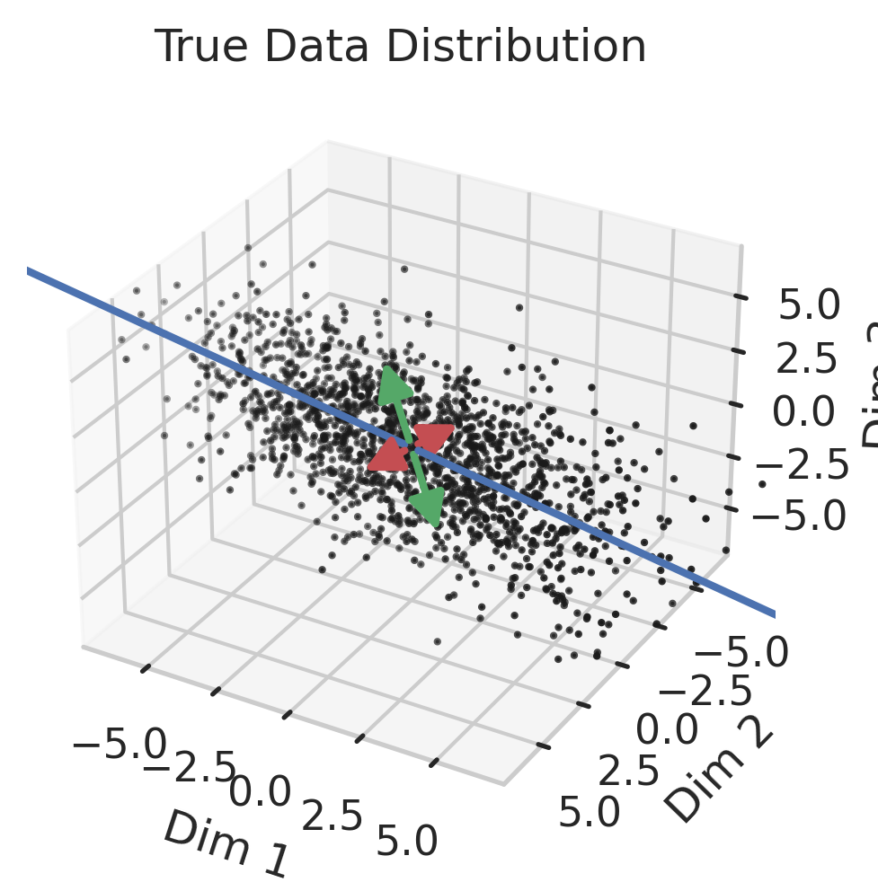
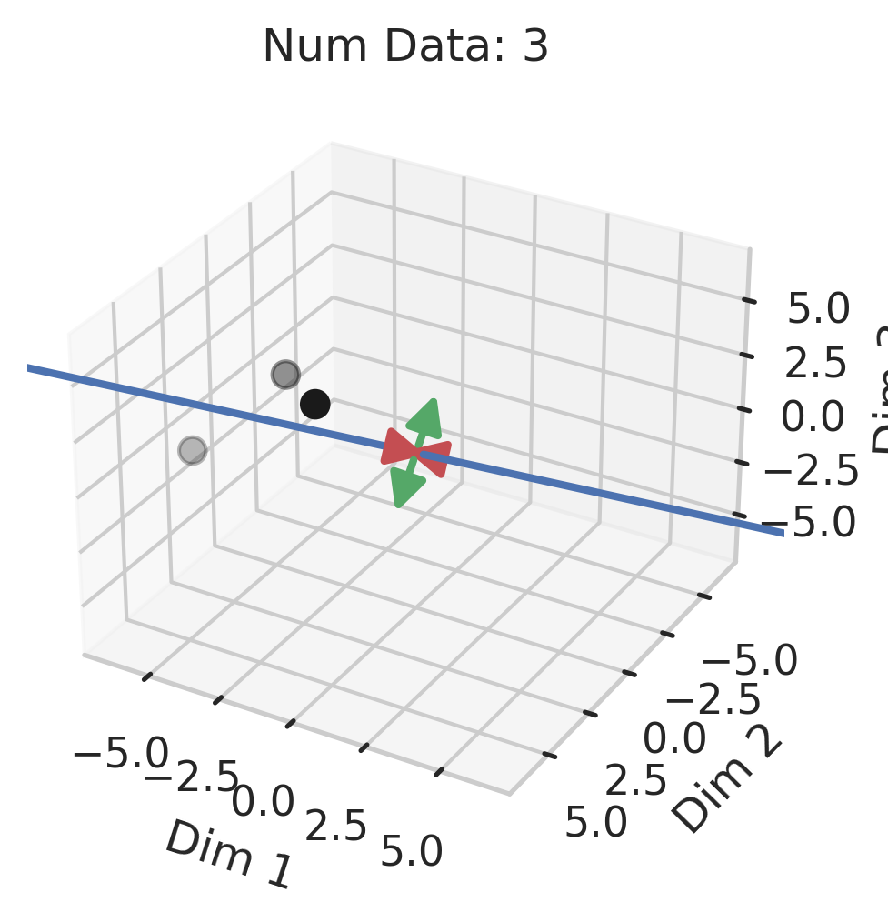
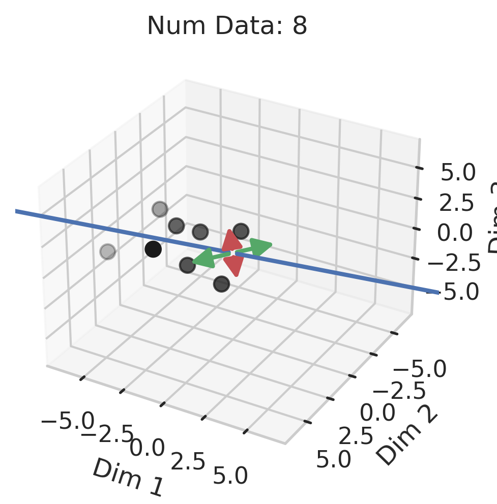
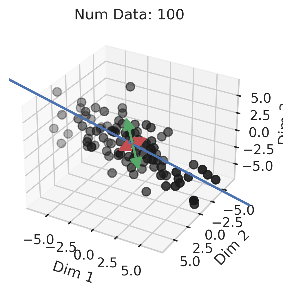
We use the term “vary” when discussing $\vec{v}_r$ because $V$ can be related to the empirical (or sample) covariance matrix oftentimes studied in Principal Component Analysis. That is, if the SVD of $X$ is $U S V^T$, then $\frac{1}{N} X^T X = \frac{1}{N} V S^2 V^T$. If the training data are centered (a common preprocessing step), then this is the empirical covariance matrix and its eigenvectors $\vec{v}_1, …, \vec{v}_R$ identify the orthogonal directions of variance. We’ll return to this in Fig 6.
Why does the test error diverge? When (1) and (3) are both present in the learning problem, the model’s parameters along this singular mode are likely incorrect. When (2) is added to the mix by a test datum $\vec{x}_{test}$ with a large projection along this mode, the model is forced to extrapolate significantly beyond what it saw in the training data, in a direction where the training data had an error-prone relationship between its predictions and the training targets, using parameters that are likely wrong. As a consequence, the test squared error explodes!
Factor 1 - Low Variance in Training Features
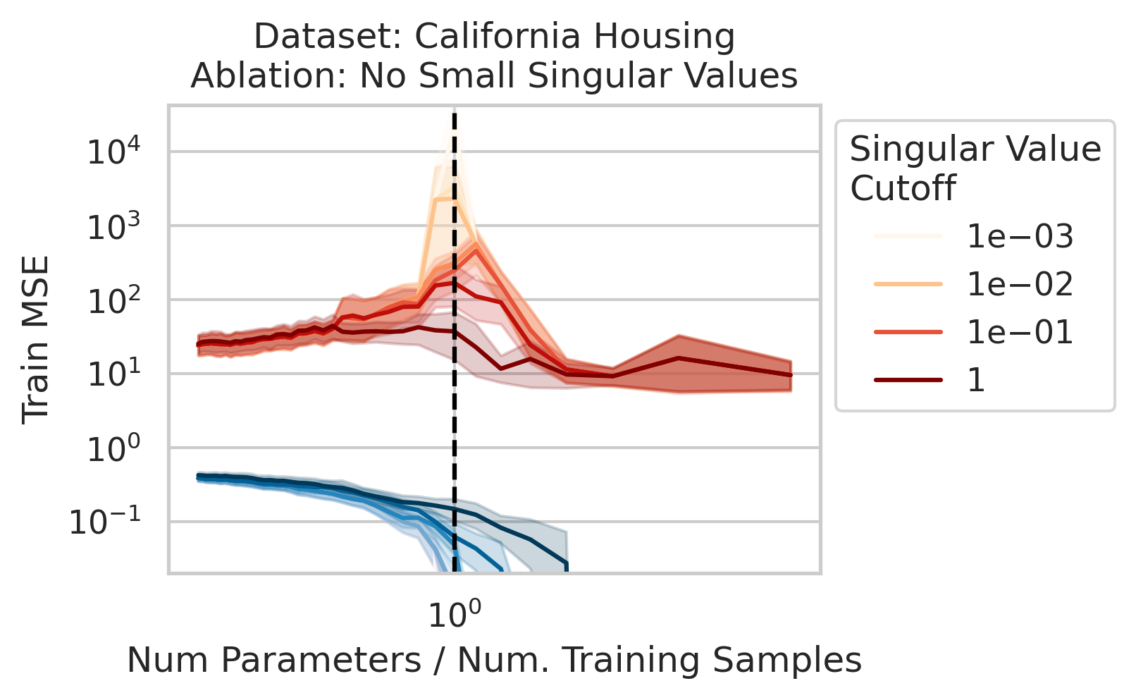
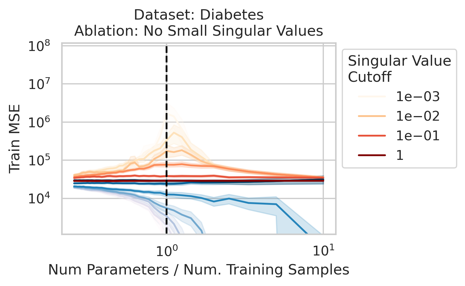
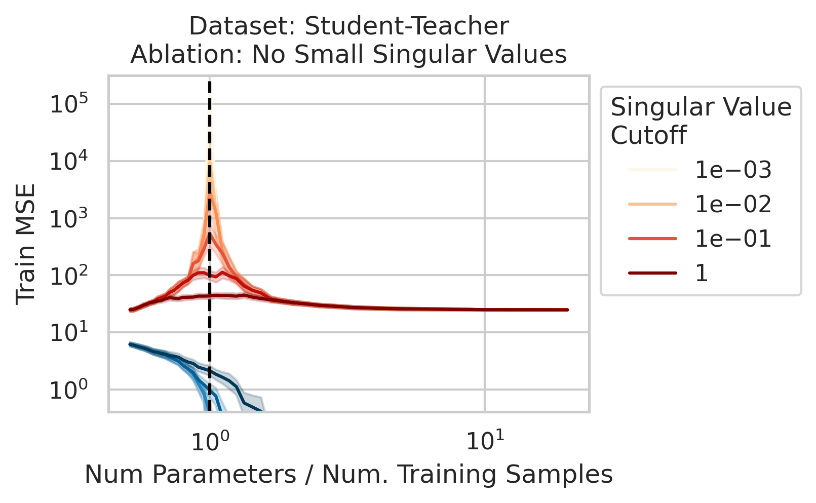
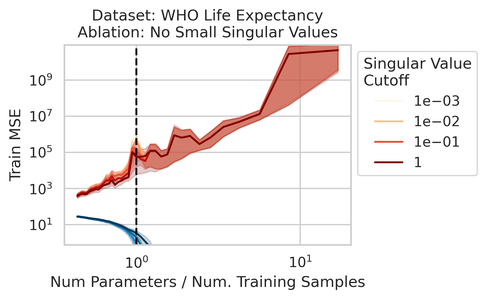
The test loss will not diverge if any of the three required factors are absent. What could cause that? One way is if small-but-nonzero singular values do not appear in the training data features. One way to accomplish this is by setting all singular values below a selected threshold to exactly 0. To test our understanding, we independently ablate all small singular values in the training features. Specifically, as we run the ordinary linear regression fitting process, and as we sweep the number of training data, we also sweep different singular value cutoffs and remove all singular values of the training features $X$ below the cutoff (Fig 2).
Factor 2 - Test Features in Training Feature Subspace

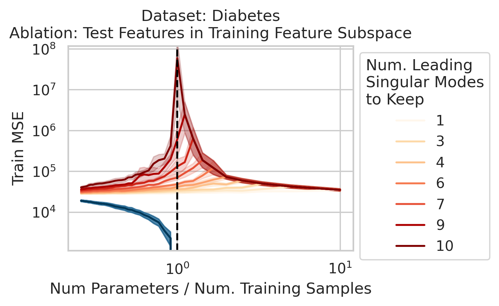


Double descent should not occur if the test datum does not vary in different directions than the training features. Specifically, if the test datum lies entirely in the subspace of just a few of the leading singular directions, then the divergence is unlikely to occur. To test our understanding, we force the test data features to lie in the training features subspace: as we run the ordinary linear regression fitting process, and as we sweep the number of training data, we project the test features $\vec{x}_{test}$ onto the subspace spanned by the training features $X$ singular modes (Fig 3).
Factor 3 - Errors from Best Possible Model
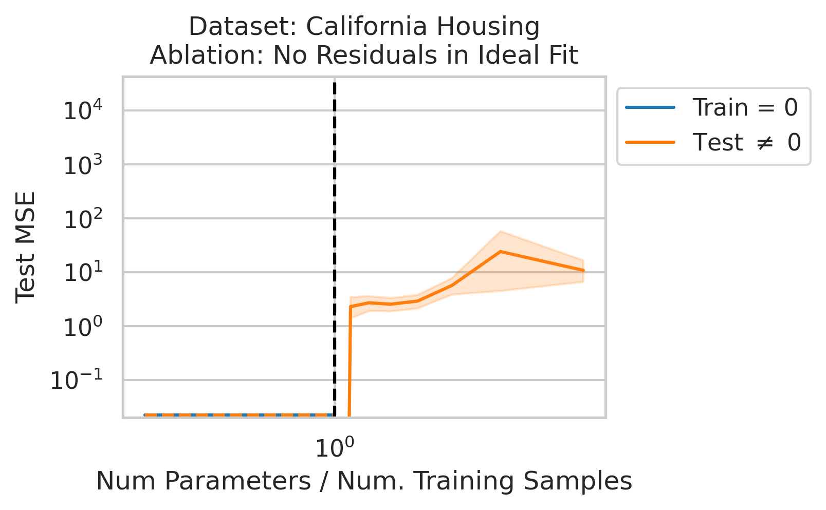
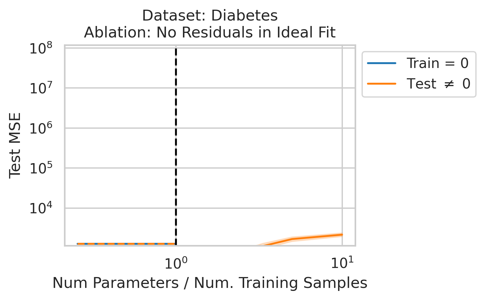
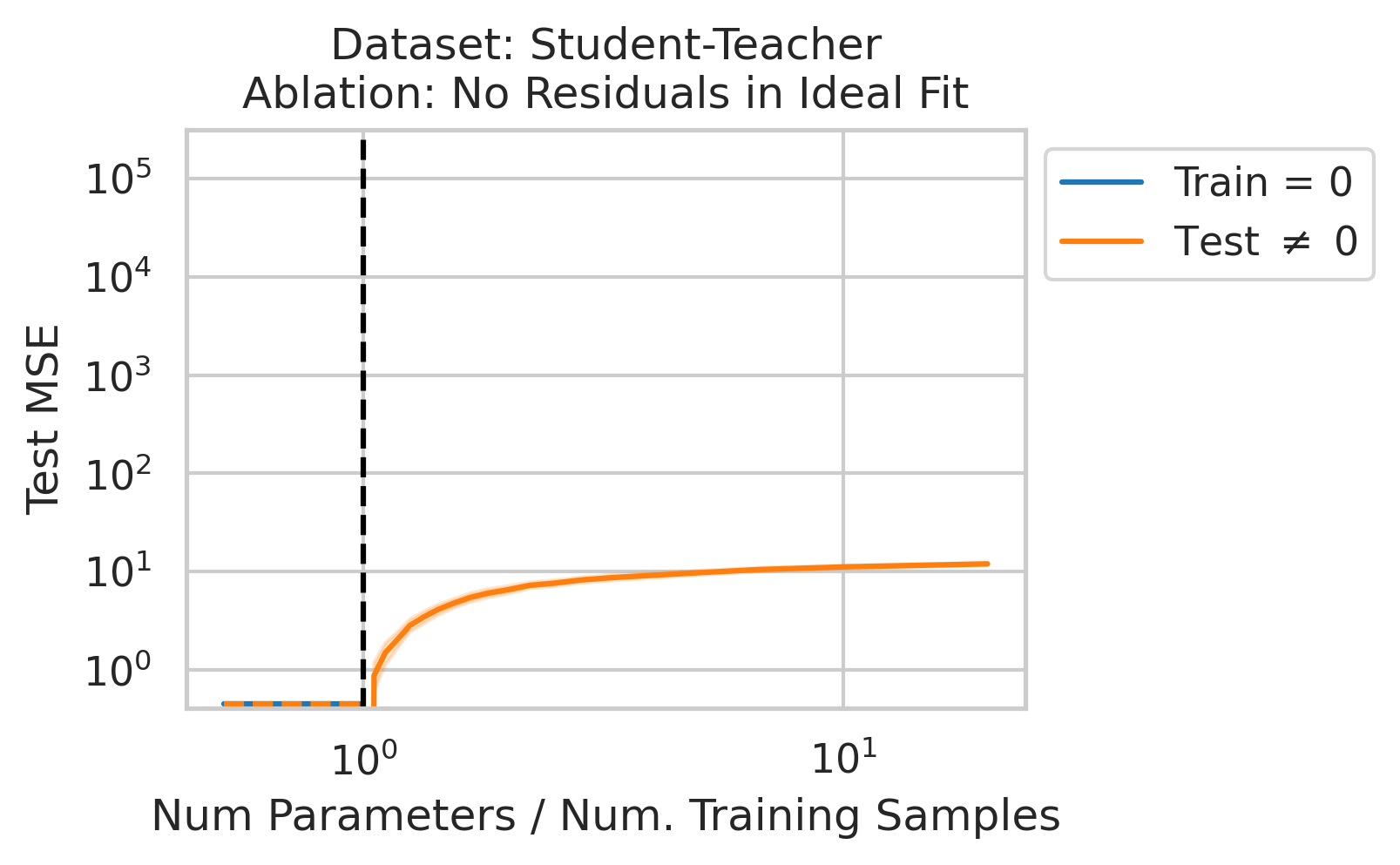
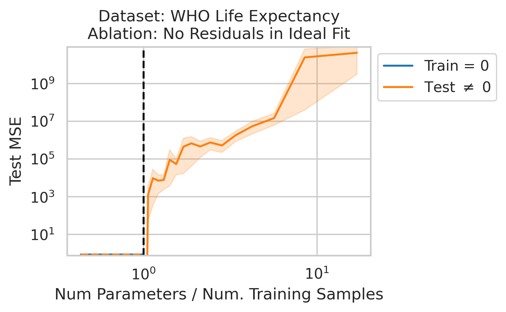
Double descent should not occur if the best possible model in the model class makes no errors on the training data. For example, if we use a linear model class on data where the true relationship is a noiseless linear relationship, then at the interpolation threshold, we will have $D=P$ data, $P=D$ parameters, our line of best fit will exactly match the true relationship, and no divergence will occur. To test our understanding, we ensure no residual errors exist in the best possible model: we first use the entire dataset to fit a linear model, then replace all target values with the predictions made by the ideal linear model. We then rerun our typical fitting process using these new labels, sweeping the number of training data (Fig 4).
As a short aside, what could cause residual errors in the best possible model in the model class?
- Noise: If the data is noisy, then the best possible model in the model class will have residual errors.
- Model Misspecification: If the data is generated by a nonlinear model, but we use a linear model class (or vice versa), then the best possible model in the model class will have residual errors.
- Missing Features: Even if the data is noiseless and our model belongs to the correct model class, but we are missing covariates, then the best possible model in the model class will still have residual errors.
Divergence at the Interpolation Threshold
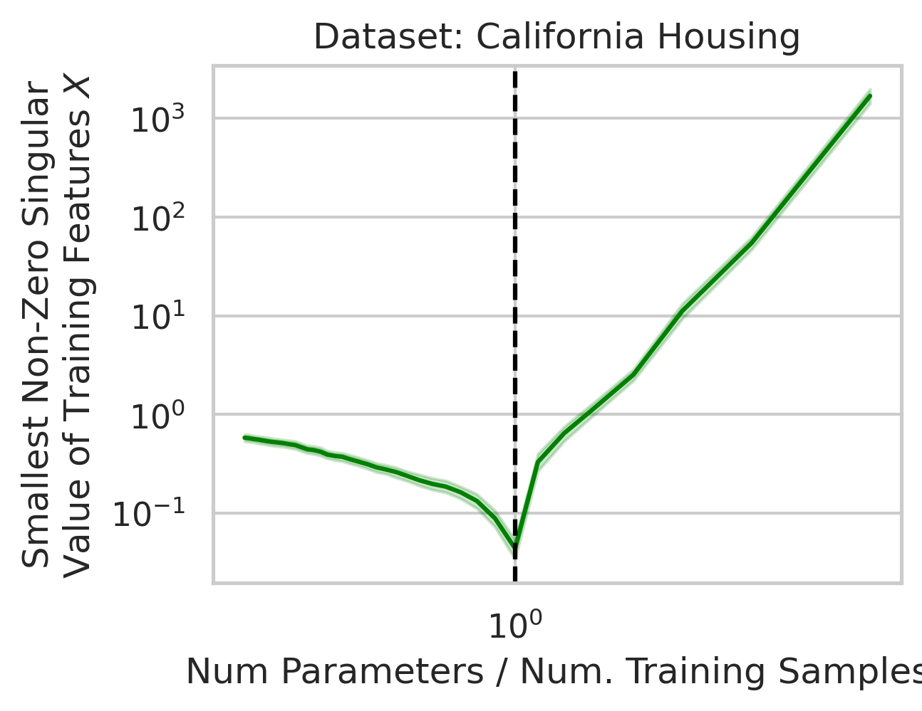
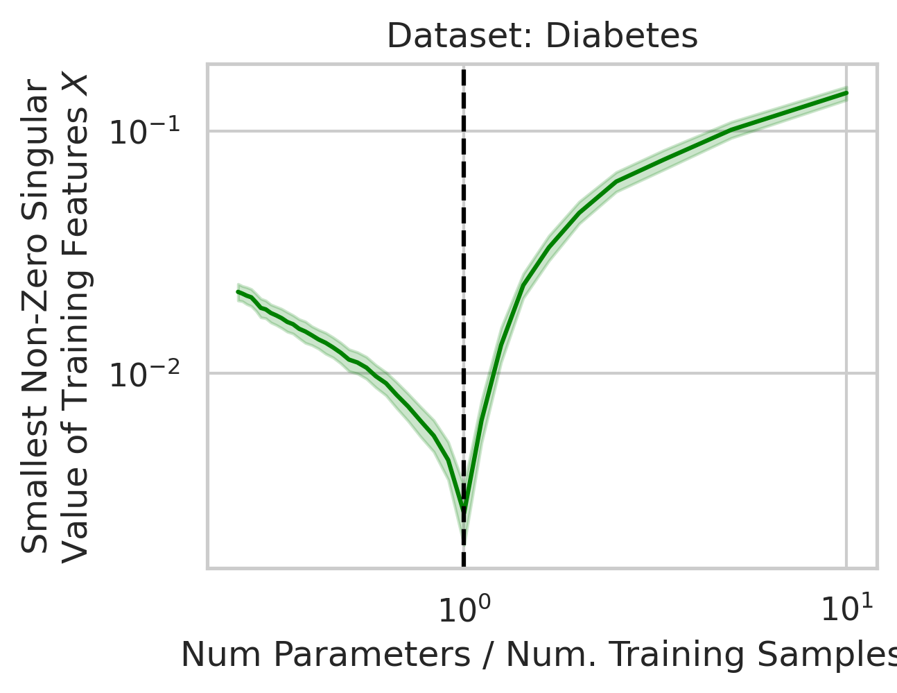


Why does this divergence happen near the interpolation threshold? The answer is that the first factor (small non-zero singular values in the training features $X$) is likely to occur at the interpolation threshold (Fig 5), but why?
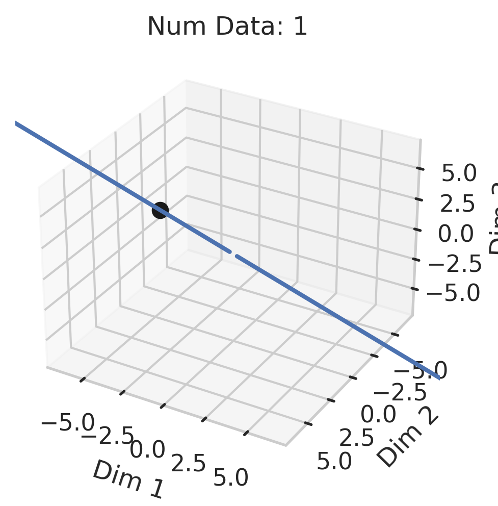
Suppose we’re given a single training datum \(\vec{x}_1\). So long as this datum isn’t exactly zero, that datum varies in a single direction, meaning we gain information about the variance in that direction, but the variance in all orthogonal directions is exactly 0. With the second training datum \(\vec{x}_2\), so long as this datum isn’t exactly zero, that datum varies, but now, some fraction of \(\vec{x}_2\) might have a positive projection along \(\vec{x}_1\); if this happens (and it likely will, since the two vectors are unlikely to be exactly orthogonal), the shared direction gives us more information about the variance in this shared direction, but less information about the second orthogonal direction of variation. Ergo, the training data’s smallest non-zero singular value after 2 samples is probabilistically smaller than after 1 sample. As we approach the interpolation threshold, the probability that each additional datum has large variance in a new direction orthogonal to all previous directions grows unlikely (Fig 5), but as we move beyond the interpolation threshold, the variance in each covariate dimension becomes increasingly clear.

Generalization in Overparameterized Linear Regression
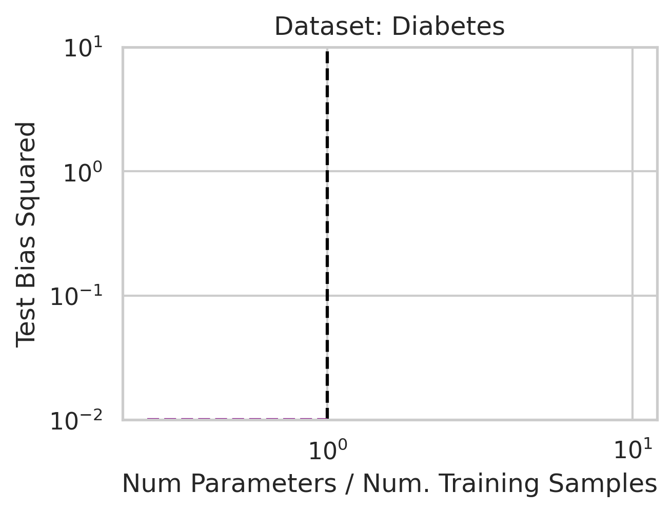
You might be wondering why three of the datasets have low test squared error in the overparameterized regime (California Housing, Diabetes, Student-Teacher) but one (WHO Life Expectancy) does not. Recall that the overparameterized regime’s prediction error has another term \(\hat{y}_{test,over} - y_{test}^*\) not present in the underparameterized regime:
\[\begin{equation} \vec{x}_{test} \cdot (X^T (X X^T)^{-1} X - I_D) \beta^*. \label{eq:bias} \end{equation}\]To understand why this bias exists, recall that our goal is to correlate fluctuations in the covariates $\vec{x}$ with fluctuations in the targets $y$. In the overparameterized regime, there are more parameters than data; consequently, for $N$ data points in $D=P$ dimensions, the model can “see” fluctuations in at most $N$ dimensions, but has no ``visibility” into the remaining $P-N$ dimensions. This causes information about the optimal linear relationship $\vec{\beta}^*$ to be lost, thereby increasing the overparameterized prediction error.
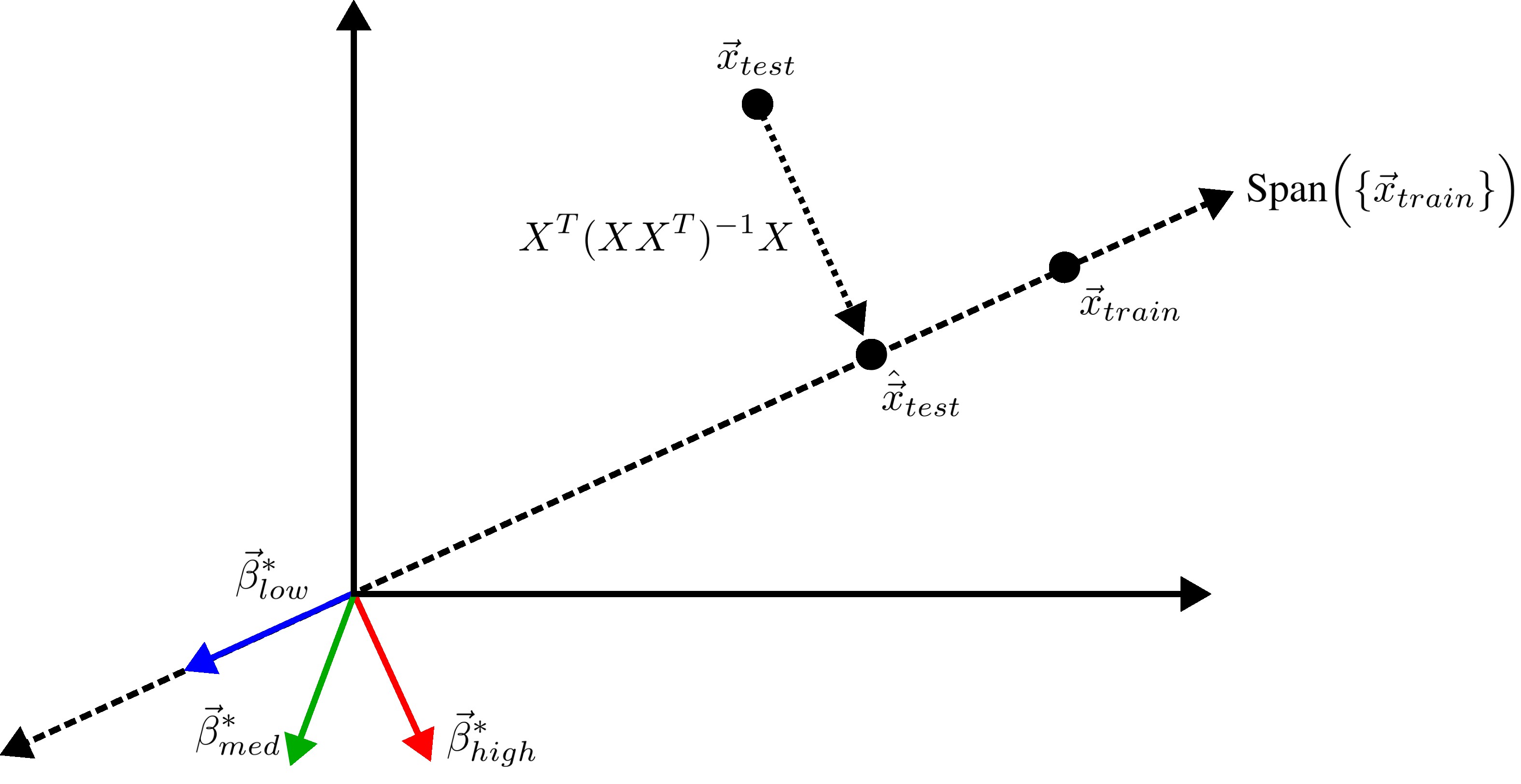
We previously saw that away from the interpolation threshold, the variance is unlikely to affect the discrepancy between the overparameterized model’s predictions and the ideal model’s predictions, meaning most of the discrepancy must therefore emerge from the bias (Eqn. \ref{eq:bias}). This bias term yields an intuitive geometric picture (Fig 7) that also reveals a surprising fact: overparameterized linear regression does representation learning! Specifically, for test datum \(\vec{x}_{test}\), a linear model creates a representation of the test datum \(\hat{\vec{x}}_{test}\) by orthogonally projecting the test datum onto the row space of the training covariates \(X\) via the projection matrix \(X^T (X X^T)^{-1} X\):
\[\begin{equation*} \hat{\vec{x}}_{test} := X^T (X X^T)^{-1} X \; \vec{x}_{test}. \end{equation*}\]Seen this way, the bias can be rewritten as the inner product between (1) the difference between its representation of the test datum and the test datum and (2) the ideal linear model’s fit parameters:
\[\begin{equation}\label{eq:overparam_gen_bias} (\hat{\vec{x}}_{test} - \vec{x}_{test}) \cdot \vec{\beta}^*. \end{equation}\]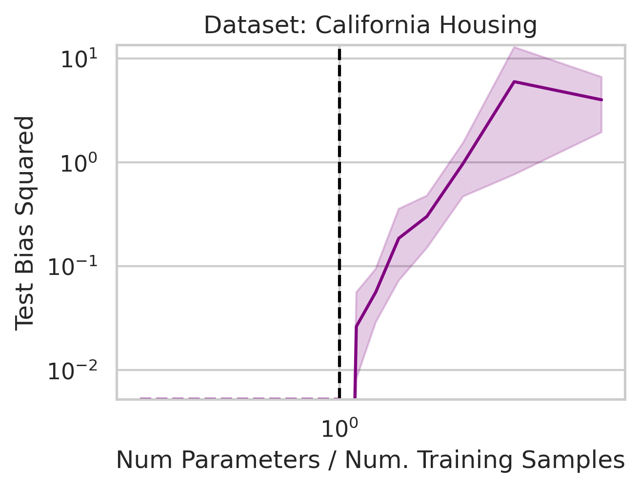
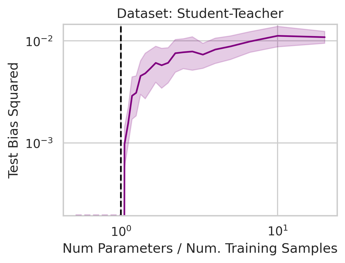

Intuitively, an overparameterized model will generalize well if the model’s representations capture the essential information necessary for the best model in the model class to perform well (Fig. 8).
Adversarial Test Data and Adversarial Training Data
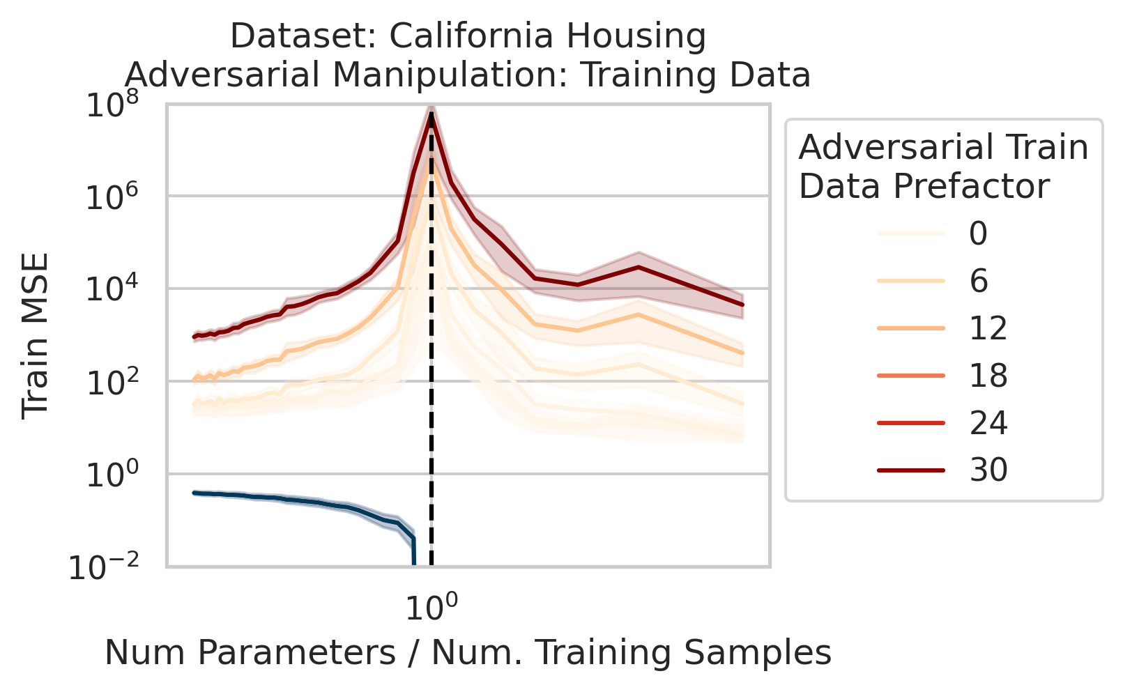
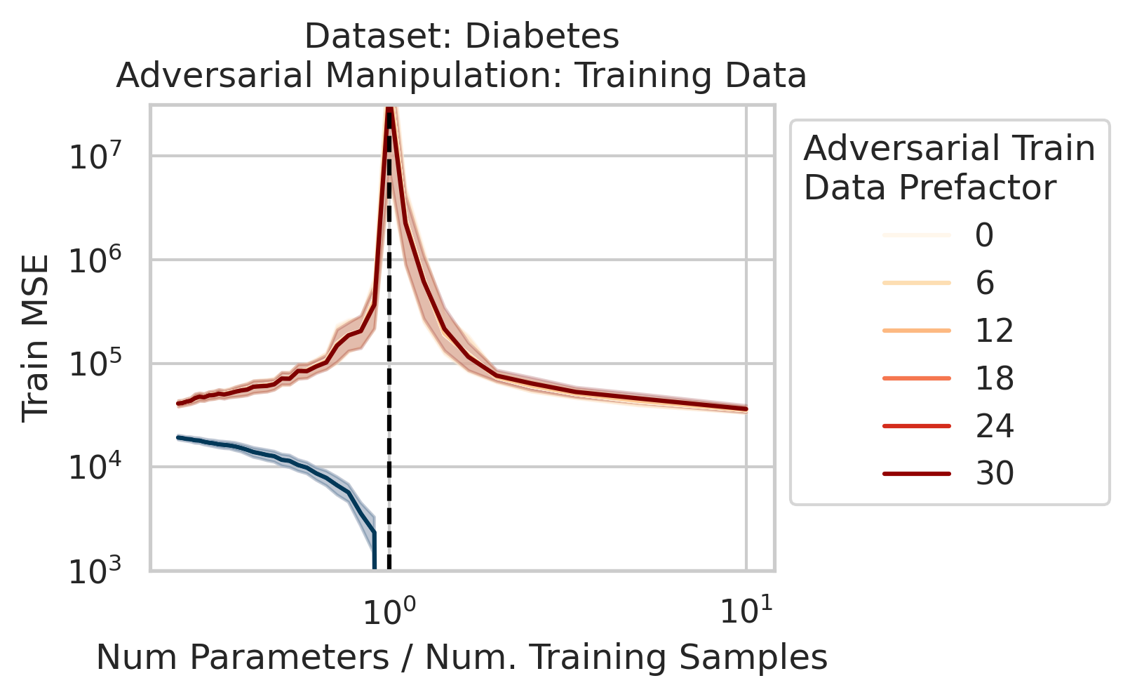
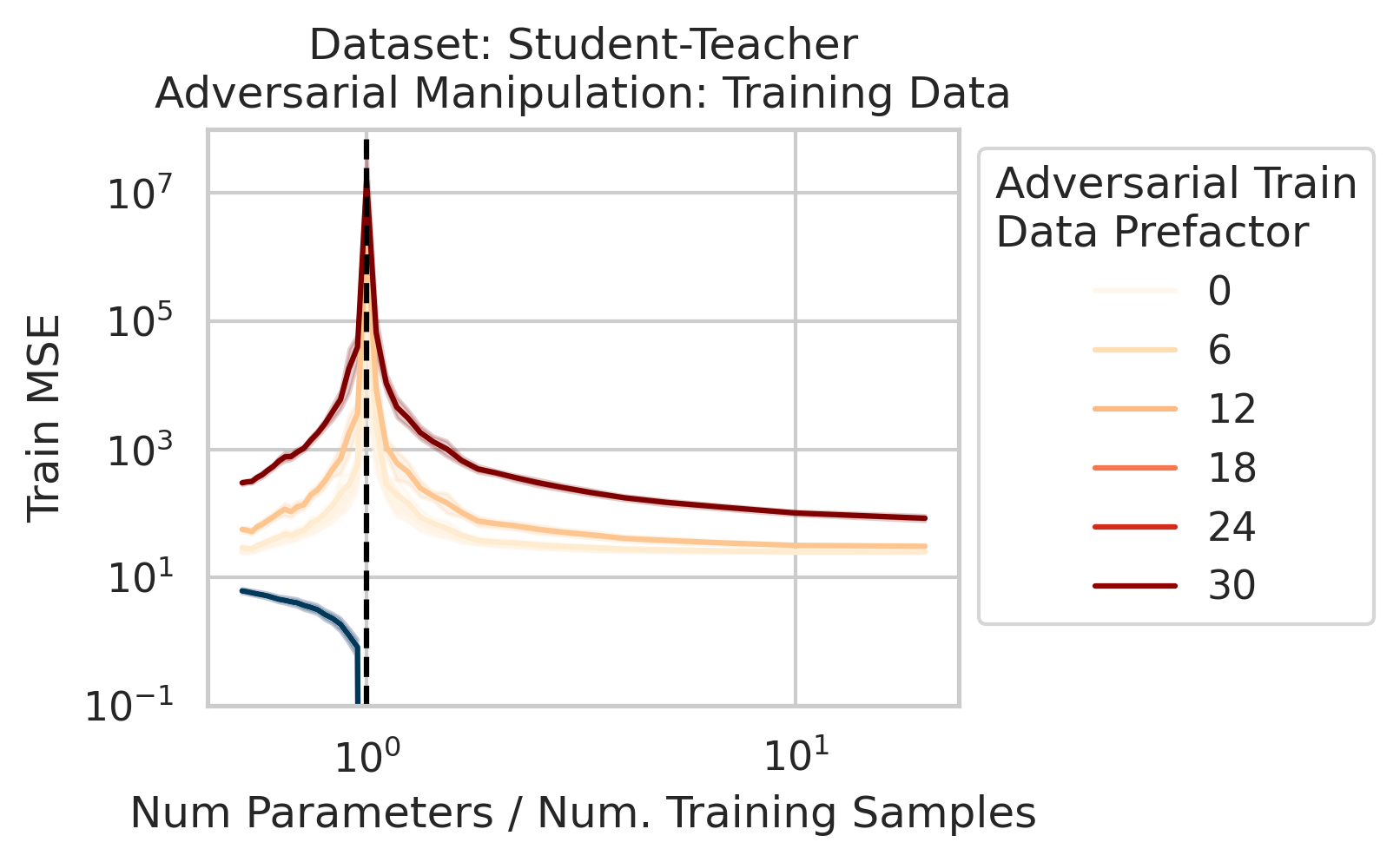
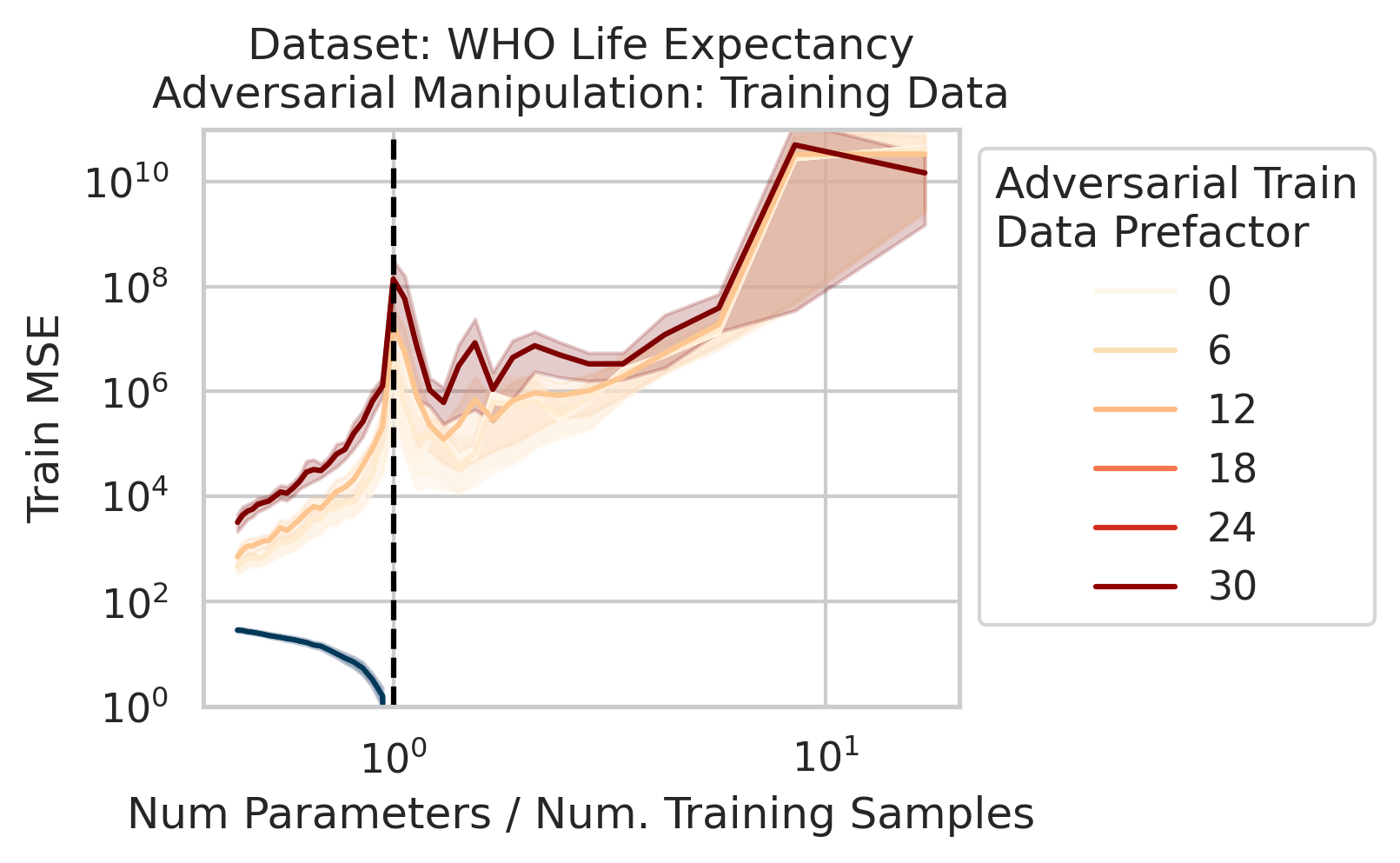
Our key equation (Eqn. \ref{eq:variance}) also reveals why adversarial test data and adversarial training data exist (at least in linear regression) and how mechanistically they function. For convenience, we repeat the equation:
\[\begin{equation*} \sum_{r=1}^R \frac{1}{\sigma_r} (\vec{x}_{test} \cdot \vec{v}_r) (\vec{u}_r \cdot E). \end{equation*}\]Adversarial test examples are a well-known phenomenon in machine learning

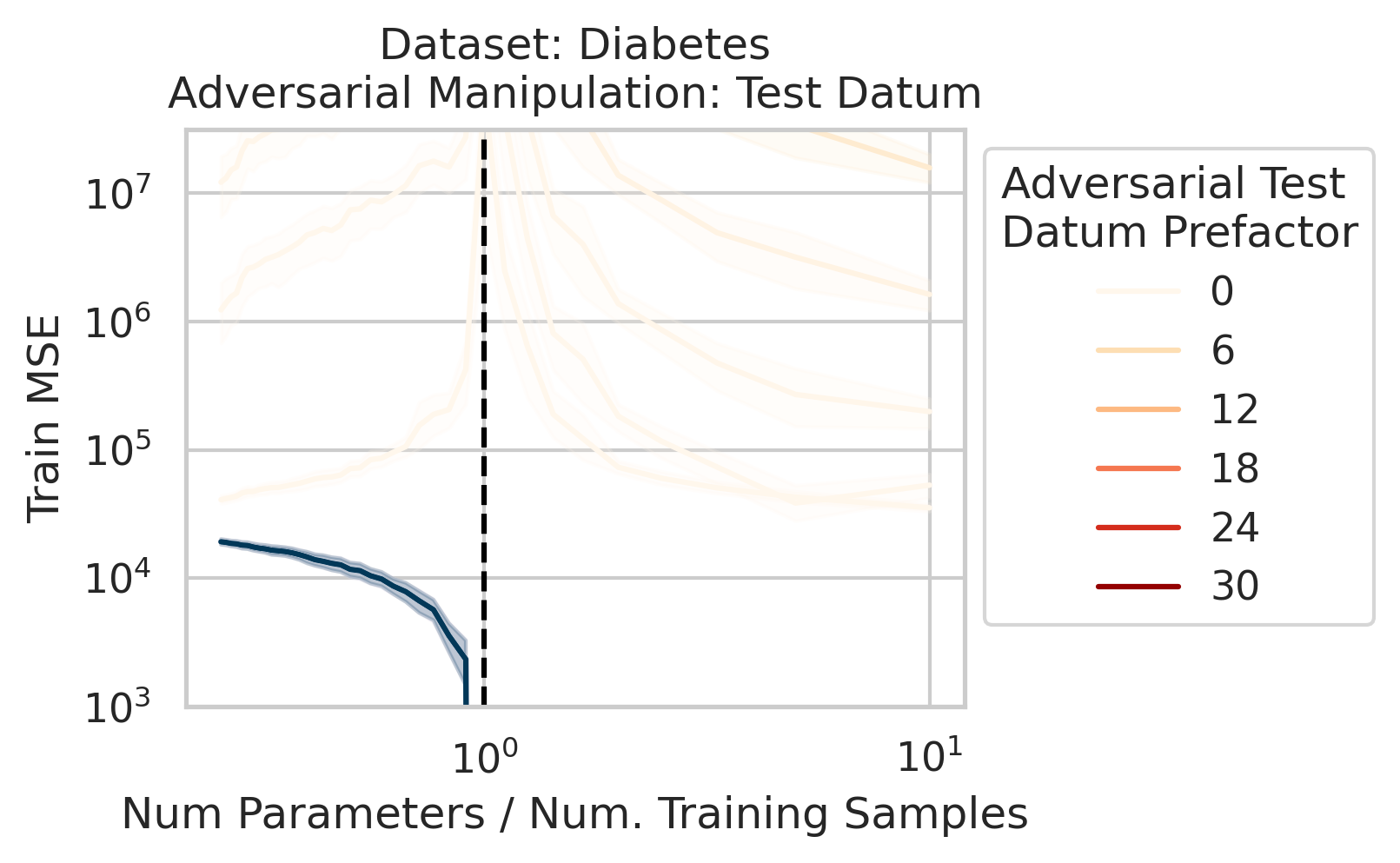
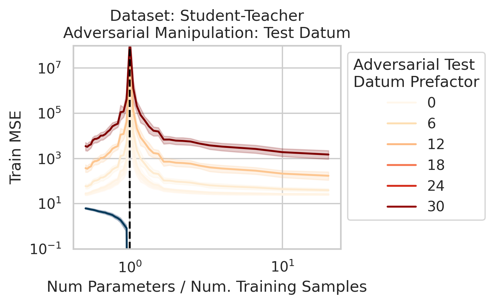
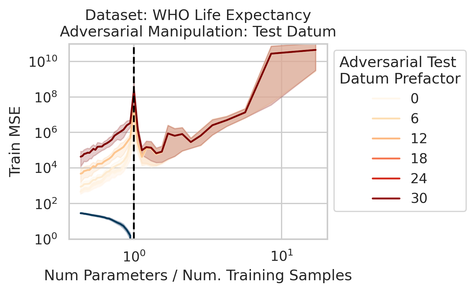
Less well-known are adversarial training data, akin to dataset poisoning
Intuition for Nonlinear Models
Although we mathematically studied ordinary linear regression, the intuition for why the test loss diverges extends to nonlinear models, such as polynomial regression and including certain classes of deep neural networks
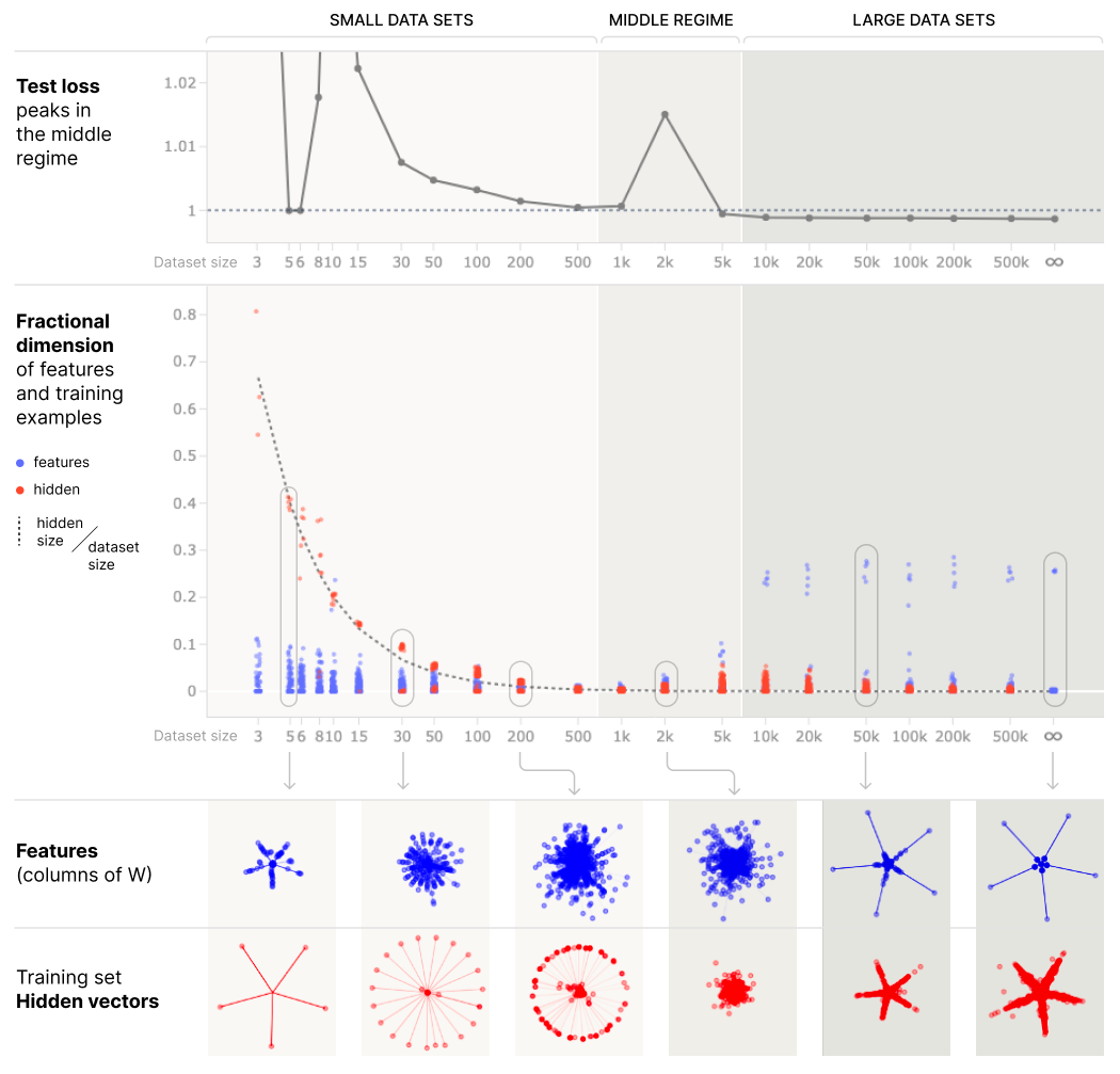
Our work sheds light on the results in two ways:
-
Henighan et al. 2023 write, “It’s interesting to note that we’re observing double descent in the absence of label noise.” Our work clarifies that noise, in the sense of a random quantity, is not necessary to produce double descent. Rather, what is necessary is residual errors from the perspective of the model class ($E$, in our notation). Those errors could be entirely deterministic, such as a nonlinear model attempting to fit a noiseless linear relationship, or other model misspecifications.
-
Henighan et al. 2023 write, “[Our work] suggests a naive mechanistic theory of overfitting and memorization: memorization and overfitting occur when models operate on ‘data point features’ instead of ‘generalizing features’.” Our work hopefully clarifies that this dichotomy is incorrect: when overparameterized, data point features are akin to the Gram matrix $X X^T$ and when underparameterized, generalizing features are akin to the second moment matrix $X^T X$. Our work hopefully clarifies that data point features can and very often do generalize, and that there is a deep connection between the two, i.e., their shared spectra.
Conclusion
In this work, we intuitively and quantitatively explained why the test loss misbehaves based on three interpretable factors, tested our understanding via ablations, connected our understanding to adversarial test examples and adversarial training datasets, and added conceptual clarity of recent discoveries in nonlinear models.