Deep Equilibrium Models For Algorithmic Reasoning

In this blogpost we discuss the idea of teaching neural networks to reach fixed points when reasoning. Specifically, on the algorithmic reasoning benchmark CLRS the current neural networks are told the number of reasoning steps they need, which they shouldn't be given. While a quick fix is to add a termination network that predicts when to stop, a much more salient inductive bias is that the neural network shouldn't change its answer any further once the answer is correct, i.e. it should reach a fixed point. This is supported by denotational semantics, which tells us that while loops that terminate are the minimum fixed points of a function. We implement this idea with the help of deep equilibrium models and discuss several hurdles one encounters along the way. We show on several algorithms from the CLRS benchmark the partial success of this approach and the difficulty in making it work robustly across all algorithms.

What is Algorithmic Reasoning?

Broadly, algorthmic reasoning studies how well neural networks can learn to execute classical computer science algorithms. In particular to measure how well an algorithm has been learned we look at size-generalisation, i.e. if we train on inputs of size $N$ and check how well the Neural Network perform on inputs of size $2N$ or $10N$. The idea is that neural networks often learn shortcuts that work well in-distribution, but fail out-of-distribution, whereas classical computer science algorithms work no matter the input size. The purpose of this exercise is to study the generalisation of reasoning tasks, especially what tricks help to improve robustness and get the network closer to deducing logically rather than relying on statistical short cuts.

Why care about fixed-points?

First, let’s remember that for $x_0$ to be a fixed-point of a function $f$ it must satisfy $f(x_0) = x_0$. Secondly, we can observe that many algorithms consist of an update rule that you apply until there is no more change. The final output can easily be seen to be a fixed-point! In a classical computer science algorithm some smart person will have sat down and shown that under some conditions on the input this convergence will happen and the final answer is correct.

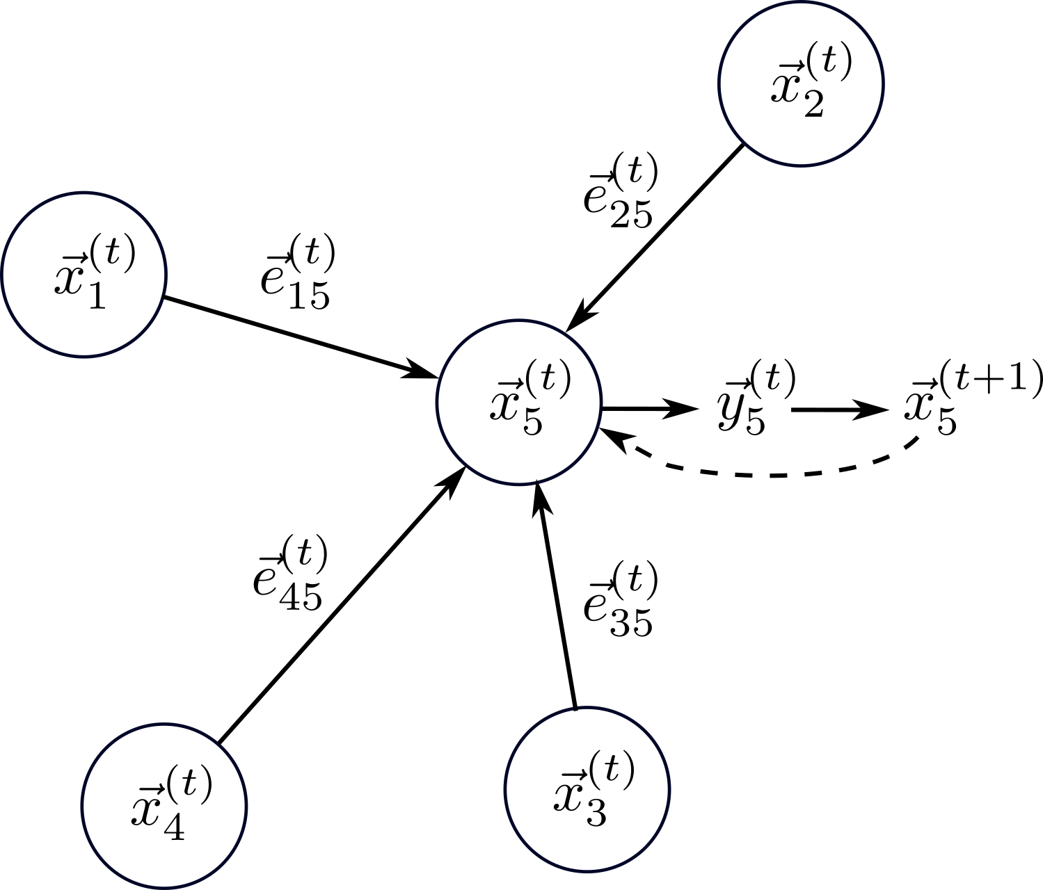
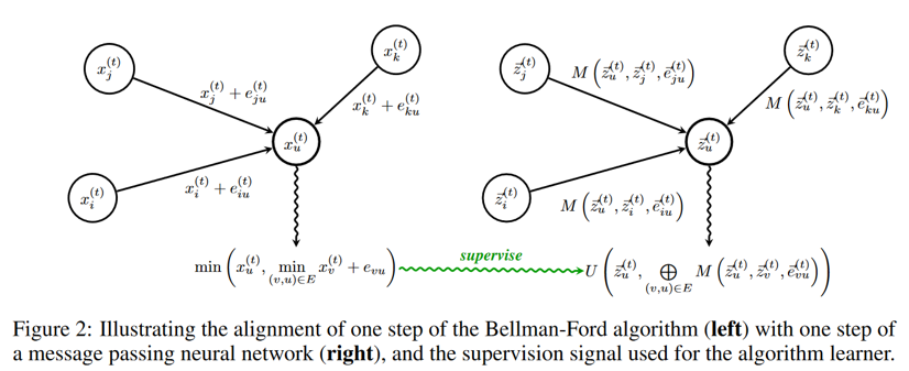
An example algorithm would be the Bellman-Ford algorithm to compute the shortest-distance to a given node in a graph. Here the update rule looks like $x_i^{(t+1)} =\min(x_i^{(t)}, \min \{x_j^{(t)} + e_{ij}\}_{j\in N(i)})$, where $x_i^{(t)}$ is the shortest distance estimate to the source node at time $t$, $e_{ij}$ is the distance between nodes $i$ and $j$, and $\{j\}_{j\in N(i)}$ are the neighbours of node $i$. The algorithm says to apply this rule until there is no more change—a fixed point.

Interestingly, denotational semantics—a theoretical field of computer science—has shown you can represent Turing complete programming languages as mathematical functions. This is mostly quite trivial with the exception of the while loop (which is also the key ingredient to make it Turing complete). Here the trick is a special mathematical operator that returns the minimum fixed point of a function! (If there is no fixed point to a function then the corresponding while loop doesn’t terminate.) And thus we can see that fixed-points are reached by all programs that terminate, and yet they aren’t used in neural networks that try to learn how to do reasoning. A missed inductive bias perhaps?

The details

Task specification

The CLRS paper provides us with a benchmark dataset for algorithmic reasoning. The general structure of the data is a sequence in time of intermediate states of a given algorithm. In other words, at timestep $t$ we have a state $x_t$ that describes various variables that the algorithm stores, e.g. in BellmanFord $x_t$ will contain the current estimate of the shortest path in each node of the graph. At each timestep $t$ we then try to predict the next time step, we do this by outputting some $y_t$ from which we can extract $x_{t+1}$. Note that $y_t$ may be slightly different from $x_{t+1}$, for instance because it has some state may never change by definition, e.g. the graph in BellmanFord, hence we don’t predict it again. This is all illustrated in the next figure, where we split the state into a state at each node $x$ and at each edge $e$ for a given graph $G$ as an example.

Algorithmic Reasoning Task, diagram recreated from

The architecture

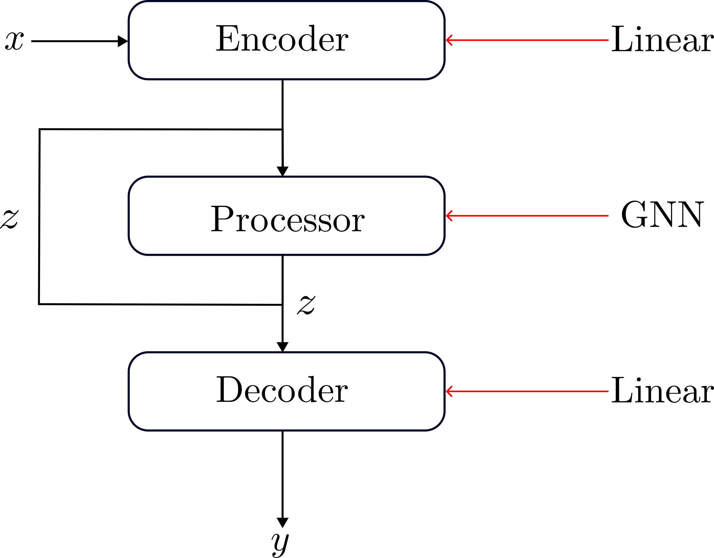
The high-level architecture is that of an encoder-processor-decoder. The motivation is that neural networks perform well in high-dimensional spaces but that classical algorithms tend to operate on very low-dimensional variables, e.g. in BellmanFord the shortest distance would be a single scalar. Thus the encoder projects the state into a high-dimensional space $z_t$ where the main computation is then done by the processor network—typically a Graph Neural Network. The output of the processor $z_{t+1}$ is then decoded back into the low-dimensional space by the decoder. The encoder and decoders mostly consist of linear layers with the occasional exception, e.g. a softmax for categorical variables. The processor will be a graph neural network, for which several different architectures have been explored, for example in. We either use the TripletMPNN from which adds edge message passing or a simple MPNN with a linear message layer.

High-level architecture employed

The processor is supposed to do the main computation of the network, in particular, the hope is that one iteration of the processor is equal to one iteration of the algorithm. In our example of BellmanFord, it would be one iteration of the update rule $x_i^{(t+1)} =\min(x_i^{(t)}, \min \{x_j^{(t)} + e_{ij}\}_{j\in n(i)})$ (see also the Figure below). Thus, the processor should indicate termination by no longer changing it’s output $z$.

Training

Traditionally the training approach has been teacher-forcing. In teacher forcing we train each step of the algorithm independently by feeding the network the ground-truth $x_t$ and computing the loss against $y_t$ at all $t$ simultaneously. This requires us to know the exact number of steps in the algorithm a priori. In other words, training with just teacher forcing will require us to tell the network the number of iterations it should run for at test time (which will vary depending on the input state). This is unrealistic in practice, where we would simply give our neural network the input state and ask it to run the algorithm on its own, which includes knowing when to stop the computation. While a termination network is suggested in , the issue is ignored in later papers such as .

Remember that neural networks are really good at learning in-distribution shortcuts. To more rigorously test whether the neural network has learned the underlying logical algorithm we introduce a shift between the training and test distribution. If the network has learned the classical algorithm, it should be able to overcome this shift. Throughout the CLRS algorithmic reasoning benchmark size generalisation is used, i.e. we train on examples of size 16 (i.e. the graph has 16 nodes) and at test time we will use an input size of 64.

An example algorithm: Bellman-Ford

How can we do fixed-points in DNNs?

One approach to training neural networks that run until they reach a fixed point is deep equilibrium models (DEQ). We give a brief introduction to this approach next based on the blogpost .

Given our input $x$, our hidden state $z$, and our processor $f$, the goal is to optimise the fixed point $z^*=f(z^*,x)$ we reach. The question how can we backprop through $z^* = f(z^*,x)$.

In backprop, we ultimately want to compute

\[\left(\frac{\partial z^*(.)}{\partial(.)}\right)^{\top} g\]

for some incoming gradient $g$ from the layers after (in our case from the decoder) and $(.)$ being anything we want, but usually the weights of the network. We can show by implicit differentation of $z^* = f(z^*,x)$ that

\[\left(\frac{\partial z^*(.)}{\partial(.)}\right)^{\top} g = \left(\frac{\partial f(z^*, x)}{\partial (.)}\right)^{\top}\left(I-\frac{\partial f(z^*, x)}{\partial z^*}\right)^{-\top}g\]

The difficult to term to solve in the above equation is $\left(I-\frac{\partial f(z^*, x)}{\partial z^*}\right)^{-\top}g$, which is the solution of a linear system, namely:

\[\left(I-\frac{\partial f(z^*, x)}{\partial z^*}\right)^{\top}h = g\]

In general, we can try to solve it in two ways, use a linear system solver, like can be found torch.linalg, or by computing a fixed point to

\[h = \left(\frac{\partial f(z^*, x)}{\partial z^*}\right)^{-\top}h +g\]

In the DEQ blogpost they suggest solving the above fixed point. The reason to use implicit differentiation is that backpropagating through time may easily run into exploding or vanishing gradients or error accumulation due to the number of steps needed to reach a fixed point.

We tried both: solving the linear system with torch.linalg.solve and finding the above fixed point. But we converged to computing the fixed point of the equation above as suggested by the deep equilibrium blogpost as it is computationally faster, while the added accuracy of linear system solvers wasn’t beneficial. Note this trade-off is heavily informed by what is readily implemented in PyTorch to run on GPU, hence the balance may shift in the future.

Tricks we employ

To encourage convergence we change the update function in the MPNN to be a minimum update, i.e. $z^{(t+1)} = \min(z^{(t)}, z^{'(t+1)})$. This update rule is motivated by the problem of getting neural networks to converge to a fixed point. We discuss the effect of this in more detail after the experimental section.

Currently, gradient flows through the implicit differentiation explained above as well as back in time through standard backprop via $z_t$. To enable more ways for the gradient to inform early steps in the algorithm, we propagate the gradient through $y_t$ as well. For discrete $y_t$, in other words, for categorical variables in the state $x_t$ we employ the Rao-Blackwell straight-through gumbel softmax estimator to allow gradients to flow.

Finally, we also try adding a loss for the number of steps by adding the penalty $\sum_{t=0}^{T} \|z_{t+1} - z_{t}\|^2$. The penalty will be larger as we take more steps and stay away from the fixed point, thus hopefully encouraging convergence to a fixed point more quickly.

How well does it work?

In the table below we show the accuracyWhat exactly is measured for the accuracy depends on each algorithm, but usually is a pointer, e.g. in the Bellman-Ford algorithm it is a pointer to the previous node along the shortest path. For more details see the CLRS Benchmark paper. of the algorithms when tested on graphs of size 64.

DEQ is our approach of reaching a fixed point together with the implicit differentiation explained above. Hint propagation is simply reaching a fixed point and back propagating through time with no implicit differentiation. Teacher forcing is used for the baselines, where the first number is the simple MPNN architecture and the second number is the more complex TripletMPNN (these numbers are taken from the paper ). For BellmanFord and BFS we use the simple MPNN and for all others we use the TripletMPNN.

Tables	DEQ	Hint propagation	Teacher forcing
BellmanFord*	96.4%	96.7%	92%/97%
Dijkstra	78.8%	84.4%	92%/96%
BFS*	53.8%	57.1%	100%/100%
DFS	5.0%	4.7%	7%/48%
MST-Kruskal	82.3%	82.3%	71%/90%
MST-Prim	75.2%	50.4%	71%/90%

As we can see in the table above the approach works very well for simpler algorithms such as BellmanFord, where with simple MPNN we manage to achieve equal or better accuracy than the simple MPNN and match the TripletMPNN. Interestingly, this is a parallel algorithm, i.e. all node representations run the same code, in constrast sequential algorithms which go through the graph node by node. We did try gating to enable the GNN to better mimic a sequential algorithm, but this didn’t help.

On the other algorithms while we are able to learn we cannot match the performance of teacher forcing where we assume to know the number of timesteps to run the neural network. This additional help makes the comparison slightly unfair, however, it shows how learning a fixed point is difficult for the network as we are not able to match the performance. We hypothesise about the reasons behind this in the next section.

What’s the problem?

There are a few major issues that we notice during training. The first is that the network is prone to underfitting, while we only show the test accuracy in the table above the training error doesn’t actually reach 0. It is unclear what causes this, however, trying to solve some issues with the DEQ may solve this. So let’s delve into them.

Convergence is a key issue

Firstly, the network will often take a large number of steps to reach a fixed point. We can see on easier algorithms like the BellmanFord algorithm that the number of forward steps during training often reaches our set upper limit of 64 forwards steps (the actual algorithm would take on average 4-5, max 10 for this graph size). This is why we implement our architecture trick, where we update the next hidden representation only if it is smaller than the current one, i.e. $z^{(t+1)} = \min(z^{(t)}, z^{'(t+1)})$ where $z^{'(t+1)}$ is the output of our min aggregator in the message passing step (alternatives such as gating and an exponential moving average update function were also tried). This helps with convergence, which enables finding a fixed point in simple cases, but fails to work reliably for more complex architectures and problems, while also introducing a different issue.

The problem with hard constraints to achieve convergence

Remember that during the implicit differentiation we are trying to solve

\[h = \left(I-\frac{\partial f(z^*, x)}{\partial z^*}\right)^{-\top}g\]

i.e. in the linear system $y = Ax$ our matrix $A$ is equal to $I-J$ where $J$ is the Jacobian in the above equation. If the Jacobian is equal to the identity then our matrix $A=0$ and our system has no solution. In practice, $z^{(t+1)} = \min(z^{(t)}, z^{'(t+1)})$ will reduce to $f(z) = z$ in many dimensions of $z$. This leads to many rows of the Jacobian being the identity due to the function effectively becoming $f(x)=x$ in many dimensions. Thus leading to rows that are entirely zero in $A$, which is ill-defined and has no solution causing the optimisation to break.

One solution is to try a soft-min, i.e. $softmin_{\tau}(a,b) = \frac{ae^{-a/\tau}+be^{-b/\tau}}{e^{-a/\tau}+e^{-b/\tau}}$. Here we get the ability to trade off between convergence and the Jacobian being interesting. For $\tau<<1$ we basically recover the min operation and for $\tau>>1$ we simply get an average, i.e. an exponential moving average. In practice, there was not a trade-off for which we consistently have an interesting Jacobian, while also converging sufficiently fast.

What do we take away?

Training to reach a fixed point can work as way to determine when to stop reasoning. But it gets increasingly more difficult as the underlying problem gets harder.
It’s unclear what inductive bias to choose in order to ensure fast enough convergence to a fixed point. There are downsides such as uninformative gradients at the fixed point.
Optimisation is tricky and stands in the way. In particular, with implicit differentiation through the fixed point.