On Bayesian Model Selection: The Marginal Likelihood, Cross-Validation, and Conditional Log Marginal Likelihood

Introduction

Model selection is a crucial aspect of machine learning, as it allows us to choose the most appropriate model for a given task. In the Bayesian setting, the marginal likelihood has been a popular tool for model selection and hyperparameter learning, often motivated by the principle of Occam’s razor. However, the suitability of the marginal likelihood depends on the specific context and goals of the modeling task.

Recently, the paper “Bayesian Model Selection, the Marginal Likelihood, and Generalization” by Lotfi et al. (2022), which was accepted as Outstanding Paper and Long Oral at ICML 2022, examined the importance and challenges of model selection in machine learning, focusing on the log marginal likelihood (LML) and proposing a variant: the conditional log marginal likelihood (CLML). The authors argue that while LML is a useful tool for hypothesis testing, it may not be the best metric for model selection and for predicting the generalization performance of trained models or learning hyperparameters. They introduce the CLML as a potential improvement and demonstrate its effectiveness across various settings, including density models, Fourier features, Gaussian Processes, and deep neural networks.

In this blog post, inspired by the above paper, we (re-)derive insights that challenge the conventional focus on the marginal likelihood and related quantities for Bayesian model selection. We argue that the quantities we examine are all consequences of Occam’s razor, and thus no single quantity should be considered universally superior. Instead, the choice of model selection criterion should be guided by the context and the desired outcomes. We highlight that many recently proposed metrics for model selection, including CLML, are closely related to cross-validation and have failure cases that can be explained by considering model misspecification and prior-data conflicts. Overall, the choice between these metrics should be based on the specific requirements of the task at hand.

We begin by discussing the foundations of model selection, including the role of Occam’s razor and its relationship to maximum likelihood estimation (MLE) and maximum a posteriori (MAP) estimation. We then introduce the concepts of log marginal likelihood (LML), cross-validation, and conditional log marginal likelihood (CLML), highlighting their connections and differences. Through a series of thought experiments and empirical observations, we explore the behavior of these model selection criteria in various scenarios, such as under model misspecification, prior-data conflict, and in different data regimes. We find that the conditional marginal cross-entropy, which is closely related to cross-validation, is often a more reliable choice when the primary objective is to select for generalization performance. On the other hand, the conditional joint marginal cross-entropy (permutation-invariant negative CLML) may be preferable when the focus is on sequential prediction and online learning. At the same time, the joint marginal information (negative LML) is rarely the right choice for model selection. We review relevant literature, including the work of Fong and Holmes (2020) on the connection between the LML and cross-validation, the training speed estimators by Lyle et al. (2020) and Ru et al. (2021), and the experiments of Lotfi et al. (2022) , comparing the CLML and validation loss for deep neural networks (DNNs). These studies provide valuable insights into the strengths and limitations of different model selection criteria.

Throughout the post, we emphasize the importance of considering the context, available data, and desired outcomes when selecting the most appropriate metric for model selection and hyperparameter tuning. By questioning the primacy of the (conditional) joint marginal likelihood and encouraging critical thinking about the foundations of these quantities, we hope to foster a more nuanced understanding of Bayesian model selection.

(Bayesian) Model Selection

In our daily lives, we’re often faced with choices that require us to sift through competing explanations or decisions. Imagine you hear your doorbell ring. You might think it’s the delivery you’ve been waiting for, a neighbor dropping by, or perhaps you didn’t hear anything at all, and it was just your imagination. In deciding between these options, you’re likely to lean towards the simplest explanation that aligns with your expectations—say, the long-awaited delivery. This inclination towards simplicity has a formal counterpart in scientific discovery and machine learning, known as Occam’s razor:

This concept is further illustrated using an example from chapter 28 of David MacKay’s seminal book, “Information Theory, Inference, and Learning Algorithms”, where the essence of selecting between models based on their evidence is laid out succinctlyBut see also:from this Reddit thread (with thanks to Freddie Bickford-Smith) that shows that the simplest explanation is always highly context- and prior-dependent..

But how can we express this formally using mathematics?

In the next section, we will use information-theoretic concepts to formalize Occam’s razor and connect it to the maximum likelihood estimation (MLE) and maximum-a-posteriori (MAP) estimation approaches. This formalization highlights that Occam’s razor, as a general principle favoring simplicity, can motivate various techniques, not just Bayesian ones. Therefore, using Occam’s razor as the sole justification for Bayesian model selection may not be as compelling as it initially appears.

However, one could argue that when Occam’s razor is properly applied within a Bayesian framework, it captures a more nuanced notion of complexity. From this perspective, the Bayesian formulation of Occam’s razor favors models that strike a balance between goodness-of-fit and model complexity, where complexity is measured by the model’s ability to compress the data. This view is consistent with the minimum description length (MDL) principle, which posits that the best model is the one that minimizes the total description length of both the model and the data given the model.

From Philosophical Principle to Mathematical Statement

Let’s first connect Occam’s razor to Maximum-A-Posteriori (MAP) Estimation and Maximum Likelihood Estimation (MLE) before diving deeper into the background and (Bayesian) model selection.

In information theory, the information content of an event \(x\) is defined as \(-\log_2 \pof{x}\), where \(\pof{x}\) is the probability of that event occurring according to a given model. This is also called Shannon’s information content. We use the base \(2\) for logarithms and measure information in bits (binary digits), and for the rest of the post, we will drop the base of the logarithm. The information content measures the optimal encoding length in bits for the event \(x\) under the model specified by its probability distribution \(\pof{\cdot}\).

Variables that cannot be directly observed are called latent variables within the context of probabilistic modeling. Occam’s razor suggests that we should prefer simpler explanations for latent variables, given the observed data.

Consider a model with a latent variable \(z\) and observed data \(x\). The model specifies a probability distribution \(\pof{z \given x}\). According to Occam’s razor, we prefer simpler explanations, which correspond to smaller values of \(-\log \pof{z \given x}\). Using Bayes’ theorem, \(\pof{z \given x} = \frac{\pof{x \given z} \pof{z}}{\pof{x}}\), we can rewrite this as:

Given that \(\pof{x}\) is independent of \(z\), we can omit it from our objective. Additionally, if we posit a uniform (or non-informative prior) for \(z\), implying that all potential values of \(z\) are equally probable before observing \(x\), then \(\pof{z}\) becomes constant and can also be dropped from our objective. This simplifies our preference to:

Equivalently, we can maximize \(\pof{x \given z}\), which is the likelihood of the observed data \(x\) given the latent variable \(z\). When making a decision and selecting a single value for \(z\), this leads to the maximum likelihood estimation (MLE) approach.

In summary, the connection between Occam’s razor and MLE relies on the following assumptions:

1. Shannon’s information content is how we measure complexity.
2. The prior distribution for the latent variables is uniform (or uninformative).
3. Simpler explanations, as measured by the information content, are preferred (Occam’s razor).

Under these assumptions, the preference for simpler explanations leads to the MLE approach, where more likely values of the latent variable given the observed data are preferred.

Optimizing the MLE is common in machine learning because we can directly optimize the likelihood function. Still, this is not easy for deep learning models because they have a large number of parameters and the loss function is non-convex.

Maximum-a-Posteriori Estimation

However, the assumption of a uniform or non-informative prior for the latent variables is not always valid or desirable. In many cases, we have prior knowledge about the latent variables that can be incorporated into the model. This leads to the Maximum-A-Posteriori (MAP) Estimation as an alternative to MLE.

In MAP estimation, \(\pof{z}\) is not constant, so we cannot drop it—we can still drop \(\pof{x}\), however—and we maximize the joint distribution \(\pof{z, x}\), or equivalently:

Before we go further, we need to introduce notation for information-theoretic quantities and concepts that we will use throughout the postThis next section is mostly shared with the sister post "Bridging the Data Processing Inequality and Function-Space Variational Inference..

Background: Information-Theoretic Notation and Concepts

Information theory deals with the communication and quantification of informationSee the excellent "Visual Information Theory" by Chris Olah for a visual introduction to information theory.. In this post, we use a unified information-theoretic notation to express various quantities related to probability distributions and their relationshipsIt largely follows "A Practical & Unified Notation for Information-Theoretic Quantities in ML".. Here are some key concepts we will use:

The information content of an event \(x\) is denoted as \(\Hof{x}\) and is defined as \(-\log_2 \pof{x}\), where \(\pof{x}\) is the probability of event \(x\) occurring. It represents the minimum amount of information needed to describe the occurrence of \(x\) given an underlying probability distribution. \(\Hof{x \given y}\) and \(\Hof{x, y}\) are analogously defined and denote the conditional and joint information content of random variables \(X\) and \(Y\), respectively. In machine learning, the information content is often used as a minimization objective, represented as the negative log-likelihood or cross-entropy when averaged over a dataset (see below).

The entropy \(\Hof{X}\) of a random variable \(X\) is the expectation of its information content:

The entropy measures the average amount of information needed to describe the random variable \(X\). It provides a measure of uncertainty or randomness associated with \(X\). We can similarly define the entropy of a conditional distribution \(\Hof{X \given Y}\) and the joint entropy \(\Hof{X, Y}\).

We will also use the Kullback-Leibler divergence \(\Kale{\pof{X}}{\qof{X}}\) and the cross-entropy \(\CrossEntropy{\pof{X}}{\qof{X}}\):

The cross-entropy quantifies the average number of bits needed to encode samples drawn from the true distribution \(\pof{X}\) using a different distribution \(\qof{X}\). The Kullback-Leibler divergence measures the difference between two probability distributions and captures the additional bits needed to encode samples from \(\pof{X}\) compared to encoding them using the true distribution \(\qof{X}\).

Expressing Occam’s Razor in Information-Theoretic Terms

Taking this notation into account, we can express Occam’s razor as:

where \(Z\) is the latent variable and \(X\) is the observed data. Note that \(x\) and \(z\) are individual realizations of the random variables \(X\) and \(Z\), respectively.

The MLE and MAP objectives are accordingly:

This measures the number of bits we need to encode the observed data given the latent variable for MLE and the number of bits to encode both the observed data and the latent variable for MAP. This relates Occam’s razor to the minimum description length principleSee the Wikipedia article on Minimum Description Length for more details..

Hyperparameter Learning and Model Selection

In many machine learning tasks, we need to determine the best hyperparameters for a model or select the most suitable model architecture from several discrete options. The primary goal is to find the hyperparameters or model that generalizes best to new, unseen data.

Both cases can be viewed as inferring a random variable \(\H\), which represents either the model choice as a categorical distribution or the hyperparameters as a continuous distribution. In this sense, \(\H\) can be considered as another latent variable in the model.

For consistency, we will continue using \(\x\) to denote data points throughout this post. Although it is common to use \(\y\) for predictions and \(\x\) for side channel information, we will not require this distinction here and will stick to \(\x\) for simplicity.

The same arguments discussed previously also apply in this context, and we can express the objective as:

Model Parameters

In addition to the hyperparameters \(\H\), we usually have model parameters \(\W\) for a given \(\h\) with a parameter distribution \(\pof{\w \given \h}\) that we need to infer based on observed data. These parameters are the learnable components of the model, such as the weights and biases in a neural network. For given \(\w\) and \(\h\), we can easily compute the likelihood \(\pof{\x \given \w, \h}\), which represents the probability of observing the data \(\x\) given the specific values of the parameters and hyperparameters. However, to make predictions or compute the marginal likelihood, we will need to consider the uncertainty in the parameter values by integrating over all possible \(\w\).

Bayesian Model Averaging

Bayesian Model Averaging (BMA) is a technique that integrates, or marginalizes, over the model parameters \(\W\) when making predictions. This accounts for the uncertainty in the model parameters, which is particularly useful when dealing with complex models, high-dimensional parameter spaces, and limited data. In contrast to the MLE or MAP estimate, which use a single parameter value \(\w\) for predictions, BMA provides a more robust and comprehensive approach. The probability of a new data point \(\x'\) under BMA is given by:

where \(\pof{\w \given \x, \h}\) is the posterior distribution of the parameters given the data, and \(\pof{\x' \given \x, \w, \h}\) is the likelihood of the new data point given the parameters, hyperparameters, and training data.

While BMA offers benefits, it is computationally challenging, particularly when dealing with high-dimensional parameter spaces commonly encountered in deep learning models. To make BMA tractable, various approximation methods, such as Markov Chain Monte Carlo (MCMC) and Variational Inference, have been proposed.

Marginal Likelihood and Estimation

Let’s now discuss the marginal likelihood and its relation to BMA. The marginal likelihood, denoted as \(\pof{\x \given \h}\), is the likelihood of the observed data given the hyperparameters, marginalized over all possible parameter values \(\W\). It is also known as the model evidence. To compute the marginal likelihood, we integrate over all possible \(\w\):

where \(\pof{\x \given \w, \h}\) is the likelihood of the data given the parameters and hyperparameters, and \(\pof{\w \given \h}\) is the prior distribution of the parameters given the hyperparameters.

Comparing BMA to the marginal likelihood, we see that they match for individual data points. However, for multiple data points (i.e., conditioning on datasets), the marginal likelihood is more complex. “BMA” typically refers to making predictions for a single new data point, while the marginal likelihood can be considered for many points simultaneously. Apart from this difference, the two are equivalent. Let’s discuss the case of multiple data points in more detail to understand why computing the marginal likelihood on datasets is even more challenging.

Datasets instead of Individual Data Points

So far, we have described everything as if we only had a single data point \(x\). However, in practice, we often have a dataset \(\xNtuple = (\x_1, \x_2, \ldots, \x_N)\).

Joint Marginal Information and Cross-Entropy

The easiest way to extend the previous definitions is to simply substitute \(\xNset\) for \(\x\) and assume we can compute a likelihood for the entire dataset using its joint predictive distribution:

We can then maximize this likelihood or equivalently minimize the joint marginal information \(\Hof{\xNtuple \given \h}.\)

If our model is exchangeable, meaning the order of the \(\x_n\) does not matter, we can equivalently take an expectation over all permutations of the data to obtain the joint marginal cross-entropy:

where \(\pdata{\cdot}\) is an empirical data distribution that allows us to draw samples without replacement. In this case, the joint marginal information and cross-entropy are equivalent.

With exchangeability, we can simply write \(\iCrossEntropy{\oppdata}{\pof{\cdot \given \h}}{\XNset}\) instead of using the tuple notation \(\iCrossEntropy{\oppdata}{\pof{\cdot \given \h}}{\XNtuple}\) as the order of the data points does not matter.

Conversely, if a model is not exchangeable, we can induce exchangeability by averaging over all permutations of the data points via ensembling. For example, deep learning models trained with stochastic gradient descent are generally not exchangeable, as the order and composition of the batches can impact the results. However, we can make them effectively exchangeable by training multiple models and averaging their predictions. In the limit of infinite models, the resulting ensemble will be exchangeableThe ensemble might not necessarily perform better though, as papers on training curricula have shown that batch order can be important..

The joint marginal cross-entropy turns a potentially non-exchangeable joint information into an exchangeable one by taking an expectation.

Marginal Information and Cross-Entropy

Before we try to understand these joint expressions, we should consider alternative ways to extend the previous definitions.

For instance, we could take the average of the likelihoods for individual data points:

Assuming an underlying data distribution \(\pdata{x}\), we can also express this as an attempt to estimate:

This provides an average score for the data likelihood.

However, from the perspective of Occam’s razor, simply taking the average likelihood is not the most principled approach. Instead, we can leverage information theory, which has been our tool of choice thus far. Recall that we prefer small values of the marginal information \(\Hof{\x \given \h}\). By taking the expectation over the data distribution, we obtain the individual marginal cross-entropy:

This cross-entropy measures the average number of bits needed to encode the data using the model’s probability distribution. As it does not involve a joint distribution, we refer to it simply as the marginal cross-entropy.

It is evident that the marginal cross-entropy and the average likelihood are not equivalent. Using the convexity of the negative logarithm and Jensen’s inequality, we see that the marginal cross-entropy is always larger than the negative logarithm of the average likelihood:

The NLL is frequently used to evaluate a model’s performance after training, typically on a held-out validation set. This is equivalent to computing the cross-entropy between the empirical distribution of the validation set and the model’s predictive distribution, conditioned on the parameters learned from the training data:

It is essential to distinguish this from the cross-entropy computed on the prior distribution of the model parameters before seeing any data, which is less useful for evaluating a trained model’s performance:

Only the NLL on a validation set conditioned on the training data provides an estimate of the model’s generalization ability after training. The same holds for the quantities marginalized over the model parameters.

Marginal Cross-Entropy vs Joint Cross-Entropy

Occam’s razor does not clearly specify which aggregate metric on \(\Hof{\x \given \h}\) we should prefer. Instead of the mean, we could use the median or a different quantile of the information content as a summary statistic to assess the model’s performance on the dataset. This might be more robust, as it is less sensitive to outliers.

Crucially, the marginal cross-entropy and related summary statistics measure the model’s performance using the “prior” parameter distribution, not the posterior conditioned on data. However, the joint distribution captures something else, which can be seen more clearly using the chain rule:

Each term is a conditional marginal information on the previous data points. Similarly, when we take an expectation over the data distribution, we obtain a chain of conditional marginal cross-entropies:

Each term in the sum is a conditional marginal cross-entropy conditioned on the previous data points, which differs from the marginal cross-entropy (recognized in the first term).

The following visualization summarizes the relationship between the conditional and joint marginal cross-entropies and information. The chain rule tells us that the area under the curve of the conditional quantities equals the joint quantity.

In summary, the marginal and joint cross-entropies offer different perspectives on a model’s performanceRecent works by Ian Osband et al., starting with The Neural Testbed: Evaluating Joint Predictions can help build intuitions for joint predictions. Similarly, a gentler introduction, comparing marginal and joint predictions, can also be found in the arXiv note Marginal and Joint Cross-Entropies & Predictives for Online Bayesian Inference, Active Learning, and Active Sampling.:

• The marginal cross-entropy and related summary statistics assess the model’s performance using the prior parameter distribution, without considering the effect of the data on the model.
• The joint marginal cross-entropy, expressed as a sum of conditional marginal cross-entropies, captures the model’s online learning performance as it processes the data sequentially.

While both metrics are useful for evaluating models, the joint marginal cross-entropy provides insight into how well the model learns from the data during training. The conditional marginal cross-entropy, on the other hand, is more suitable for assessing the model’s generalization ability at a given point in time, without the influence of parameter updates.

Intermediate Comparison

Regarding the earlier question of what metric we should prefer and use for model selection, let’s consider:

1. The marginal cross-entropy, as in the first term, is likely not useful for model selection with deep learning models, as it is not conditioned on any data and thus cannot correlate well with the model’s performance after training.

2. If we care about the model’s “generalization” performance after training on \(N-1\) data points without further adaptation, the marginal cross-entropy on the last data point is the more relevant quantity:

   \[\iCrossEntropy{\oppdata}{\pof{\cdot \given \h}}{\X_N \given \X_{N-1}, \ldots, \X_1}\]

   It measures the model’s performance on the last data point after having seen all previous data points, similar to a “leave-one-out” metric. Indeed, it is equivalent to leave-one-out cross-validation when we have an empirical data distribution consisting of \(N\) data points and sample without replacement.

3. More generally, it is equivalent to cross-validation when we hold out more than one data point for evaluation from the empirical data distribution:

   \[\iCrossEntropy{\oppdata}{\pof{\cdot \given \h}}{\X' \given \X_{N-k}, ..., \X_{1}}.\]

   This is the same expression as in (2.) but we assume there are more samples to draw from in the empirical data distribution \(\pdata{\x'}\). We call this term the conditional marginal cross-entropy and keep in mind its connection to cross-validation.

4. On the other hand, if we care about the model’s performance as an online learner, or in the case of LLMs, as an in-context learner, the joint marginal cross-entropy becomes a more relevant metric. It measures the model’s ability to adapt and make accurate predictions as it sequentially processes new data points, conditioned on the information it has seen so far.

   In the context of online learning, the model receives data points one at a time and updates its predictions based on the cumulative knowledge gained from previous data points. The joint marginal cross-entropy captures how well the model incorporates this sequential information to make accurate predictions for future data points.

   Similarly, for in-context learning of LLMs, the model is provided with a prompt or context consisting of a sequence of data points, and it is expected to generate accurate completions or predictions based on this context. The joint marginal cross-entropy measures the model’s ability to effectively utilize the provided context to make accurate predictions for the next data point in the sequence.

5. However, we would not want to use the unconditional joint marginal cross-entropy, but rather condition on some initial data to be closer to the actual use case of the model, which will have been (pre-)trained already. As such, we are interested in estimating a conditional joint marginal cross-entropy:

   \[\iCrossEntropy{\oppdata}{\pof{\cdot \given \h}}{\XNsetk \given \XNkset}.\]

   By conditioning on some initial data points, this metric assesses the model’s capacity to learn and adapt its predictions based on the evolving context after already having been trained to some degree. Compared to the conditional marginal cross-entropy above, this cross-entropy provides a more fine-grained evaluation of the model’s sequential prediction performance, taking into account the specific order and dependencies within the data.

   Moreover, the conditional joint marginal cross-entropy can be used to compare different models or hyperparameter settings in terms of their online learning or in-context learning capabilities. By evaluating this metric on held-out data sequences, we can determine which model or setting is better suited for tasks that require sequential adaptation and context-dependent predictions.

6. If we have a preferred order of the data points (or a split in the case of exchangeability), we can also consider the conditional joint marginal information:

   \[\Hof{\xNsetk \given \xNkset, \h}.\]

7. Both the conditional joint marginal cross-entropy and the conditional joint marginal information can be viewed as negative “conditional log marginal likelihood (CLML)” as defined by Lotfi et al. (2022), depending on whether one takes the definition as given in the main paper, in which case it is equivalent to the conditional joint marginal information, or the permutation invariant version described in the appendix, which is equivalent to the conditional joint marginal cross-entropy.

8. All these quantities are equally valid from the perspective of Occam’s razor.

9. We have not discussed how to efficiently estimate these quantities, especially for deep learning models. More importantly, we have already considered that the joint marginal information (marginal likelihood), BMA, and the joint marginal cross-entropy (as an expectation over the marginal likelihood) are not easy to estimate.

This brings us to one of the main points:

This is a crucial point that has not been sufficiently considered in the literature on model selection and hyperparameter learning previously, where the model evidence and marginal likelihood have been presented as the ultimate criteria. In practice, we rarely update a model on additional data during inference—this is changing with the advent of LLMs and strong in-context learners, but it is still not the norm.

All in One Table

There is value in contrasting all these quantities in a single table to make the differences more apparent and build understanding. Below is a tabular overview of the key quantities discussed in the context of model selection and evaluation. As a reminder, \(\H\) are the hyperparameters, \(\W\) are the model parameters, and \(\X\) are the data points, and the empirical data distribution \(\pdata{\cdot}\) samples without replacement. We will only consider marginalized quantities, so \(\W\) is integrated out.

The building blocks of these quantities are thus:

• Marginal quantities assess the model’s performance after marginalizing over the parameter distribution;
• Joint quantities capture the model’s performance on multiple data points as a whole, taking into account the dependencies between them, which can be also viewed as the average performance during online learning when using a sequential decomposition via the chain rule;
• Conditional quantities measure the model’s performance conditioned on previously seen data points, providing insights into its generalization ability or online learning performance after some data fit has happened, which can be more meaningful.

The choice of the most appropriate metric depends on the specific context and the intended use case of the model.

But then, why has the marginal likelihood been the preferred choice for model selection so far then?

Different Data Regimes

To explore when the conditional marginal cross-entropy and joint marginal cross-entropy lead to different outcomes for model selection and hypothesis testing, let’s consider a few key scenarios.

For the discrete case, we can reduce the question to one about ranking: if we have two possible hyperparameter choices \(\h_1\) and \(\h_2\), when do we get the same ranking \(\h_1 \succ \h_2\) for both metrics?

Model Misspecification

First, let’s examine the case when we have a large amount of data available. Here, model misspecification, a common concern, plays a crucial role.

As renowned statistician George Box famously stated:

All models are wrong, but some are useful.

When working with real-world data, we must always assume that our models are misspecified to some degree. Models simplify complex systems and cannot capture every nuance of the data-generating process. Consequently, the goal of model selection is not to find the “true” model but rather to identify the most useful model that balances simplicity, interpretability, and predictive performance.

Without model misspecification, we would always converge to the maximum likelihood estimate (MLE) that matches the data-generating model in the infinite data limit as the Bernstein-von Mises’ theorem tells us that posteriors converge to the MLE in the limit. However, in practice, we are always dealing with misspecified models, and the MLE will not converge to the true data-generating model.

Infinite Data Limit

Let’s return to our question of when the different quantities lead to similar rankings.

While a conditional joint marginal cross-entropy, as a sum of conditional marginal cross-entropies, is obviously larger than each individual term, if we divide the joint marginal cross-entropy by the number of samples in the conditional joint distribution, we obtain the rateIn this context, "rate" refers to the average amount of cross-entropy or information per (training) sample, drawing parallels to the concept of entropy rate in Shannon's information theory. This usage is distinct from other common uses of "rate" in machine learning, such as learning rate or convergence rate. of the conditional joint marginal cross-entropies as its per-sample average, which can be more easily related:

Bernstein-von Mises’ theorem tells us that the posterior distribution of the model parameters converges to a normal distribution around the MLE as the number of data points goes to infinityThere are likely fewer caveats to this statement than the naive interpretation of the theorem implies because we are usually not interested in converging towards some unique and identifiable parameters but rather in the predictions matching the data-generating process.. This means that the later terms in the chain rule decomposition of the joint cross-entropy will converge to the same value in the infinite sample limit as the data we condition on becomes infinite. If we take the limit, we can ignore the first terms in the chain rule decomposition of the joint cross-entropy, and we will get the same average value for the terms of the joint cross-entropy (one per sample in the joint) and the conditional cross-entropy. This matches a similar result on entropy rates in “Elements of Information Theory” by Cover & Thomas.

Overall, we have (without formal proof):

Given sufficient data (in the infinite sample limit), we see that either of these quantities will lead to the same ranking of different hyperparameters/model hypotheses. Conversely, we can expect to see meaningful differences only in low-data regimes, where the model is not yet fully adapted to the data.

Finally, in the infinite data limit, for the conditional marginal cross-entropy, we don’t need to take an expectation over the data we condition on (as the model parameters will still have converged):

forany \(\xNset \sim \pdata{\xNset}\) as \(n \to \infty\). More importantly, this also holds for the joint marginal information, whose rate in the limit is the same as the rate of the joint marginal cross-entropy above (and thus also joint cross-entropy):

We have previously mentioned the connection between cross-validation, leave-one-out validation, and the conditional marginal cross-entropy. This result also connects the marginal likelihood in the limit to these quantities.

Thus:

The catch is that “sufficient data” might be a very large amount of data, especially for highly expressive models like neural networks.

Hence, we only expect these quantities to be meaningfully different in the low-data regime. So let’s focus on the low-data regime now.

Prior-Data Conflict

Even if different hyperparameter choices lead to the same generalization loss in the infinite data limit, they can induce different priors that affect the convergence speed and model performance in the low-data regime.

In the low-data regime, assuming all models converge to the same validation loss given infinite data, we prefer the model that converges the fastest, i.e., with the least amount of training data. A model with a prior well-aligned with the data distribution learns efficiently and generalizes better with limited data.

In this scenario, the area under the conditional marginal cross-entropy or information curve (equivalent to the joint marginal cross-entropy, or joint marginal information) indicates the preferred model. The model with the lowest joint marginal information (highest log marginal likelihood) fits the available data best while having a prior enabling efficient learning and generalization.

Anti-Correlated Model Misspecification and Prior-Data Conflict

Finally, what happens when there are both model misspecification and a prior-data conflict in the low-data regime? If both are correlated, the ranking will be preserved, but if they are anti-correlated, the ranking might change.

Let’s visualize this: the curves will intersect at some point, and the model with the best achievable loss in the infinite data limit might not be the best choice in the low-data regime, depending on how much data we can train on. The optimal model choice may also change based on the amount of available data.

Here, the joint marginal cross-entropy and the joint marginal information (log marginal likelihood) might not lead to the same decision because the area under the curve at the start might be larger than what the best model can save later. This could change the ranking of the models compared to the conditional marginal cross-entropy (leave-one-out cross-validation) at the end of training, which serves as a proxy for the model’s generalization performance.

Instead, the conditional joint marginal cross-entropy and information can shine here by conditioning “away” the beginning of the curve, thus giving us a better estimate of the conditional marginal cross-entropy (or expected information) at the point of interest.

To formalize this, we can use the chain rule to split the joint marginal cross-entropy into two terms:

Note that the per-sample averages of both terms converge to the same value in the infinite data limit—the conditional marginal cross-entropy (cross-validation loss), as discussed previously. However, the second term will converge faster because it does not include the constant \(\iCrossEntropy{\oppdata}{\pof{\cdot \given \h}}{\XNsetk}\).

We can also see both terms as approximating the conditional marginal cross-entropy (cross-validation loss) for a fixed \(N\) in the low-data regime. The per-sample average of the second term will provide a better approximation.

In summary, the consistency of the ranking will depend on the size of \(\iCrossEntropy{\oppdata}{\pof{\cdot \given \h}}{\XNsetk}\) for different \(\h\) and how it compares to the conditional joint marginal cross-entropy \(\iCrossEntropy{\oppdata}{\pof{\cdot \given \h}}{\XNset \given \XNsetk}\).

This analysis highlights the importance of considering both prior-data conflict and model misspecification when selecting models in the low-data regime. The choice of performance metric and the amount of available data can significantly impact the ranking of models. The conditional joint marginal cross-entropy provides a more accurate estimate of the model’s generalization performance by conditioning away the initial part of the learning curve, which may be heavily influenced by prior-data conflict.

Approximating the Validation Loss

You may be wondering: why bother with the marginal likelihood or conditional joint marginal cross-entropy at all? Why not just always use leave-one-out cross-validation (i.e., the conditional marginal cross-entropy) or a simple validation loss?

While that is a valid approach, the key question is: can we approximate the validation loss earlier in training, without fully training the model? Or can we do this more efficiently than performing inference on each element of a validation set?

One option is to extrapolate the training loss to predict the validation loss. While potentially underexplored in this context, scaling laws have been found effective for predicting model performance.

Alternatively, when training a model on a dataset for a single epoch—which is still surprisingly common for large language models, especially without active data sampling—the average training loss per batch provides a good approximation of the validation loss. With a cross-entropy loss, this is equivalent to estimating the conditional marginal cross-entropy.

However, the batch size may not be large enough for a precise estimate. Averaging over the last few batches or using an exponential moving average can help, as the training losses on earlier batches were computed with older model parameters. Compared to using only the last batch’s loss, this smooths the estimate and reduces sensitivity to outliers.

In the multi-epoch setting, revisiting data points multiple times prevents using the training loss as a validation loss estimate. Here, cross-validation offers a solution: train on the held-out data in the last epoch, compute the validation loss via the training losses, and obtain an ensemble of fully trained models without wasting data.

In summary, while the validation loss is the gold standard, approximations based on the training loss or cross-validation can provide efficient estimates, especially in the early stages of training or with limited data.

The Big Comparison

In this post, we have explored various metrics for model selection and hyperparameter learning in the Bayesian context, focusing on the marginal likelihood, joint marginal cross-entropy, and conditional marginal cross-entropy. Our discussion has led to several key insights:

1. Infinite Data Limit: As the dataset size approaches infinity, the rate of the log marginal likelihood (or equivalently, the joint marginal information), the joint marginal cross-entropy, and the conditional marginal cross-entropy converge to the same value when averaged over the data distribution. Given sufficient data, all these metrics will produce the same ranking of different model hypotheses or hyperparameter choices.

2. Connection to Cross-Validation: The conditional marginal cross-entropy is equivalent to the expected cross-validation loss. Cross-validation is the gold standard for model selection in machine learning practice, where a model’s generalization performance is estimated by evaluating it on held-out validation data after training on the remaining data.

3. Sufficient Data Requirement: The amount of data needed for the convergence of these metrics in the infinite data limit may be impractically large, especially for highly expressive models like deep neural networks. Therefore, the convergence property may not be directly relevant in many real-world scenarios.

4. Low-Data Regimes: When data is limited, the metrics can differ significantly. The conditional marginal cross-entropy (or cross-validation loss) is often the more reliable choice for model selection targeting generalization performance, as it directly measures the model’s ability to predict unseen data after being trained on the available data.

5. Sequential Prediction and Compression: The joint marginal cross-entropy, which corresponds to the negative log marginal likelihood, may be preferable if the focus is on a model’s overall sequential prediction performance or compression ability on the training data itself. It measures how well the model fits the entire training dataset jointly, without splitting into train and validation sets.

   Moreover, the conditional joint marginal information and cross-entropy are particularly relevant for measuring the performance of online learners and the in-context learning abilities of large language models (LLMs). These metrics capture the model’s ability to adapt and make accurate predictions based on the sequential information and evolving context after training on available data.

6. Model Misspecification and Prior-Data Conflict: In practice, models often face a combination of model misspecification (where the true data-generating process is not contained within the model class) and prior-data conflict (where the prior distribution does not align well with the data distribution). The interplay between these factors can lead to different rankings of models depending on the amount of available data and the specific metric used for evaluation.

While the marginal likelihood has been a popular tool for model selection and hyperparameter learning in the Bayesian community, its suitability depends on the specific context and goals. The conditional marginal cross-entropy, closely related to cross-validation, is often a more reliable choice when the primary objective is to optimize generalization performance. However, the conditional joint marginal cross-entropy (or conditional log marginal likelihood) may be preferable when the focus is on sequential prediction after training or measuring in-context learning abilities.

Now, after having thought about all this in detail and mostly from first principles, let’s discuss the literature and how it supports or augments these considerations.

Literature Review

Having discussed the key concepts, we will now look at several influential papers that have shaped the previous discussion on model selection and hyperparameter tuning in the Bayesian context or have provided valuable insights into the marginal likelihood and its connections to other metrics.

Fong and Holmes (2020): “On the marginal likelihood and cross-validation”

Fong and Holmes (2020) explore the connection between the log marginal likelihood (joint marginal information) and cumulative leave-p-out cross-validation. Under exchangeability, they show that the joint marginal information can be rewritten as a cumulative sum of leave-p-out cross-validation terms.

The authors define the leave-p-out cross-validation score as:

where \(\binom{[N]}{p}\) denotes the set of all \(p\)-length subsets of \(\{1,...,N\}\)—the indices of the validation set—\(\x^V_i\) is the \(i\)-th validation data point, and \(\x^{\bar{V}}_k\) is the \(k\)-th training data point. This score measures the model’s performance using \(p\) validation points given the remaining data for training, equivalent to the respective conditional marginal cross-entropy.

The cumulative leave-P-out cross-validation score is defined as:

This score focuses on the last \(P\) stages of the learning curve equally and is the same as the conditional joint marginal cross-entropy. For \(P=N\), the cumulative leave-N-out cross-validation score equals the joint marginal information:

Comparing \(P<N\) to \(P=N\), Fong and Holmes highlight the potential sensitivity of the marginal likelihood to the choice of prior. They argue for using cumulative cross-validation following a preparatory training phase with \(P<N\) (e.g., \(10\%\) or \(50\%\)), demonstrating benefits over the full marginal likelihood for model selection, especially with vague priors or model misspecification.

The paper also discusses the coherence of the log posterior predictive probability as a scoring rule in cross-validation and explores connections to prequential analysis and intrinsic Bayes factors.

Fong and Holmes (2020) strongly support the ideas in this blog post, particularly the connections between marginal likelihood, cross-validation, and focusing on later learning curve stages for model selection. They establish the equivalence between the cumulative leave-p-out cross-validation score and conditional joint marginal information, aligning with our discussion of the conditional joint marginal cross-entropy as a more reliable metric compared to the full marginal likelihood.

Lyle et al. (2020) and Ru et al. (2021): Training speed and model selection

In “A Bayesian Perspective on Training Speed and Model Selection”, Lyle et al. (2020) establish a connection between training speed and the marginal likelihood in linear models. They propose using the sum of mini-batch training losses as a proxy for the log marginal likelihood to predict the generalization behavior of deep neural networks. This sum, referred to in later works as the training speed estimator (TSE), corresponds to the area under the learning curve. For 1-sample batches, the TSE is defined as:

where \(\Hof{\x_n \given \w_n}\) is the cross-entropy loss at training step \(n\) with model parameters \(\w_n\). Thus, an MLE estimate is used instead of conditioning on the data points \(\x_{<n}\) and using the BMA.

The authors provide an iterative algorithm for linear models to estimate a lower bound on the LML over multiple epochs of training. This allows capturing the model’s performance as it sees more data points over the course of training, rather than being limited to a single epoch. They also discuss extending their estimator to the infinite-width limit of neural networks.

Building upon Lyle et al. (2020), Ru et al. (2021) focus on using TSE for model selection in neural architecture search in “Speedy Performance Estimation for Neural Architecture Search”. They propose two variants of TSE: TSE-E, which focuses on the last few epochs, and TSE-EMA, which uses an exponential moving average to assign higher weights to later epochs:

where \(\alpha \in (0, 1)\) is a hyperparameter controlling the decay rate.

The authors hypothesize that assigning higher weights to later epochs may lead to better correlation with the true generalization performance of the final trained network, as the early epochs may be unstable and less informative.

They demonstrate empirically that TSE-E and TSE-EMA can reliably estimate the generalization performance of neural architectures with a small training budget and remain effective for a large range of training epochs. TSE outperforms other efficient estimators, such as early stopping and learning curve extrapolation, in terms of rank correlation with the true test performance.

The TSE estimators proposed by Ru et al. (2021) align closely with the ideas discussed in this blog post, as they prioritize the model’s performance in the later stages of learning. The empirical results presented by Ru et al. (2021) and Lyle et al. (2020) provide supporting evidence for the importance of going beyond the marginal likelihood.

Lotfi et al. (2022): “Bayesian Model Selection, the Marginal Likelihood, and Generalization”

Lotfi et al. (2022) provide a comprehensive re-evaluation of the marginal likelihood as a metric for predicting the generalization performance of trained models and learning hyperparameters. They argue that while the marginal likelihood is well-suited for prior hypothesis testing, it is only peripherally related to generalization after training. The authors identify several practical and philosophical issues in using the marginal likelihood for selecting between trained models, such as its sensitivity to the choice of prior, potential to lead to both underfitting and overfitting, and negative correlation with generalization performance in some cases.

To address these limitations, Lotfi et al. propose the conditional marginal likelihood (CLML) as a partial remedy. The CLML is computed by conditioning on a subset of the training data, which helps to mitigate the influence of the prior and focus on the model’s performance under this posterior. It is also less sensitive to the number of parameters in the model. The authors demonstrate that the CLML is better correlated with generalization than the marginal likelihood and provides promising performance for deep kernel hyperparameter learning and neural architecture search.

The CLML shares significant similarities with the cumulative leave-p-out cross-validation score proposed by Fong and Holmes (2020). Both approaches essentially propose the same metric, which focuses on the model’s performance in the later stages of learning and provides a more reliable indication of generalization compared to the full marginal likelihood. Lotfi et al. also critically compare their work to that of Lyle et al. (2020), but do not discuss the work of Ru et al. (2021).

Lotfi et al. conduct an extensive empirical evaluation of the CLML across various settings, comparing it to the marginal likelihood and other baselines under different conditions, such as varying dataset sizes, model complexities, and hyperparameter settings. They demonstrate that the CLML consistently outperforms the marginal likelihood in terms of selecting the hyperparameters that lead to better generalization performance. The authors also acknowledge some limitations of their work, such as the need for further theoretical analysis of the CLML’s properties and the potential challenges in estimating the CLML for more complex models.

The key novelty of Lotfi et al.’s work lies in their comprehensive analysis of the limitations of the marginal likelihood for model selection and hyperparameter learning, as well as their proposal of the CLML as a practical alternative that addresses these limitations.

A Simple Toy Experiment

To illustrate the concepts discussed in this post, we conduct a simple toy experiment using a Bayesian linear regression model. The goal is to demonstrate how the various information metrics behave under different prior settings and dataset sizes, and to show that none of the metrics are universally reliable. In particular, the joint marginal information may not be the best choice when the primary concern is static performance after training on data.

Experimental Setup

We generate a synthetic dataset with 64 features and 500 training and validation samples each. The true coefficients are drawn from a normal distribution with a mean of 2, and the target is the dot product between the features and the true coefficients.

For the model, we use a Bayesian linear regression with an isotropic Gaussian prior on the weights (hyperparameter \(\wstddev\)) and independent Gaussian noise (hyperparameter \(\noisestddev\)). The model is misspecified when \(\noisestddev > 0\). We consider three different prior settings:

• Model 1 (\(\h_1\)): \(\wstddev=0.1\), \(\noisestddev=0.8\)
• Model 2 (\(\h_2\)): \(\wstddev=100\), \(\noisestddev=1.0\)
• Model 3 (\(\h_3\)): \(\wstddev=1\), \(\noisestddev=1.2\)

Thus, all three models are misspecified to varying degrees and exhibit different levels of prior-data conflict.

We train the model on subsets of the training data of varying sizes, ranging from 1 to the full training set size, performing 5 trials with different splits. For each subset size, we compute the following metrics:

• Joint Marginal Information (JMI)
• Conditional Joint Marginal Information (CJMI) with half the data used for conditioning
• Marginal Cross-Entropy (MCE) on the training set
• Marginal Cross-Entropy (MCE) on the validation set
• Training Speed (Approximate)
• Joint Marginal Information Rate (JMI Rate)

The JMI is equivalent to the negative log marginal likelihood, the CJMI to the negative conditional log likelihood, and the MCE corresponds to the cross-entropy loss. The Training Speed approximates an iterative algorithm by following the full data gradient. The JMI Rate is the JMI divided by the dataset size, which converges to the MCE in the infinite data limit.

Results

The results of the experiment are summarized in the following plots:

The plots show the behavior of the information metrics as the dataset size increases for the three different prior settings. Some key observations:

• The marginal cross-entropy (MCE) metrics decrease as the dataset size increases, indicating improved model performance.
• The joint marginal information (JMI) increases with more data, as it is equivalent to the area under the curve of the MCE on the training set. (As we take the average over multiple trials, its mean is actually an estimate of the joint marginal cross-entropy.)
• The JMI rate, which is the JMI divided by the dataset size, decreases very slowly towards the same value as the MCE. This agrees with the previous discussion on the infinite data limit.
• The training losses also decrease, while their sum, equal to the training speed estimator (TSE), increases with the dataset size.
• The conditional joint marginal information (CJMI) with half the data used for conditioning shows a similar trend to the JMI but with lower values, as it focuses on the model’s performance on the held-back data. As we take an average over multiple trials, it is actually an estimate of the conditional joint marginal cross-entropy.

To further analyze the model selection behavior, we computed the CJMI for different conditioning set sizes and selected the model with the lowest CJMI for each combination of dataset size and conditioning set size. The results are visualized in the following plot:

The plot shows which model is selected based on the lowest CJMI for different dataset sizes (x-axis) and conditioning set sizes (y-axis). The white line represents the case where half the data is used for conditioning (CJMI half in the previous plot). We observe that the model selection decision changes depending on the amount of available data and the size of the conditioning set/held-back data.

A Narrow but Deep Dive into “Bayesian Model Selection, the Marginal Likelihood, and Generalization”

Now that we have introduced the necessary concepts and discussed the literature, let’s take a closer look at the paper by Lotfi et al. (2022).

Use Cases and Pitfalls of the LML

Lotfi et al. (2022) present both the case for the log marginal likelihood (LML) as well as potential pitfalls when using it. They highlight the following use cases for the LML—quoted and paraphrased from the paper:

1. Hypothesis testing: The LML provides an elegant mechanism to select between fixed prior hypotheses, even if each hypothesis is entirely consistent with observations. It automatically favors the most constrained hypothesis that fits the data, encoding a notion of Occam’s razor. The paper gives the example of the LML favoring general relativity over alternative explanations for Mercury’s orbit.

2. Hyperparameter learning: The LML is often successfully used in practice to learn hyperparameters of the prior, finding the hyperparameters \(\h\) that maximize \(\pof{\mathcal{D} \given \h}\), where \(\mathcal{D}\) is a dataset. The paper highlights Gaussian processes as a compelling example, where the LML chooses kernel hyperparameters that make the distribution over functions likely to generate the training data, rather than simply maximizing data fit. The LML can learn many kernel parameters and be used where cross-validation would be intractable.

3. Constraint learning: Unlike typical learning objectives like maximum likelihood, the LML is incentivized to select for constraints. It provides a consistent estimator for constraints, automatically selecting the most constrained solution that fits the data and collapsing to the true constraint value as the number of observations grows. Examples include the LML consistently estimating the true dimensionality in Bayesian PCA and automatically learning symmetries like rotation invariance.

However, the paper argues that the LML has several pitfalls for model selection and generalization:

4. Not aligned with generalization: The LML answers “what is the probability a prior model generated the training data?” rather than “how likely is the posterior to have generated withheld points?”. A prior that initially explains the data well can still lead to a posterior that generalizes poorly.

5. Misaligned in model selection: The LML evaluates priors, while model selection should evaluate posteriors. Maximizing LML is not equivalent to selecting the best generalizing posterior.

6. Can overfit: The LML can favor “simple” priors concentrated around overfit maximum likelihood solutions that generalize poorly.

7. Underfitting bias in hyperparameter selection: The LML may not favor hyperparameters that make good parameters likely if they also make many poor parameters likely.

Relating these points to the previous discussions:

For hypothesis testing and hyperparameter learning (1. & 2.), the LML favors the simpler hypothesis that converges faster, implying a smaller area under the learning curve. This aligns with the discussion on prior-data conflict for similarly misspecified models.

At the same time, the paper also states about the case of Mercury’s orbit that:

We emphasize here we are comparing fixed prior hypotheses. We are not interested in how parameters of general relativity update based on orbital data, and then deciding whether the updated general relativity is the correct description of orbital trajectories.

This could be misconstrued at computing the marginal cross-entropy for the data under the prior, which is not what the LML is doing: it computes a joint marginal cross-entropy after all. The two questions in (4.) point to the joint and conditional marginal cross-entropies—the areas under the full and partial learning curves, respectively.

However, neither LML nor CLML align with static evaluation, but rather with continued learning (5.).

Points (6.) and (7.) relate to prior-data conflict and model misspecification when they are anti-correlated.

Overall, all quantities can fail in the low-data regime. In the infinite data limit, model (mis-)specification dominates other factors, making the quantities less interesting.

The “Conditional Marginal Likelihood” in Lotfi et al. (2022)

The paper introduces the conditional marginal likelihood (CLML) as a remedy for the pitfalls of the LML, matching the earlier definition of conditional joint marginal information:

Unlike the LML which is invariant to data order, the CLML depends on how the data is split into a conditioning set and validation set. To make the CLML permutation-invariant, the paper proposes averaging over different permutations, equivalent to the joint marginal cross-entropy. However, this becomes computationally expensive, so the paper uses a single permutation with \(P=20\% \, N\) to ensure the posterior has sufficiently converged.

Estimating the CLML and LML via Laplace Approximation

Computing the LML via sampling is intractable for deep neural networks. Estimating it from an uninformative prior leads to high-variance estimates, as most \(\w\) sampled from the prior will perform poorly on the data. While Monte Carlo sampling works well in high dimensions, it fails here because randomly sampling a good \(\w\) from the prior is incredibly unlikely, as illustrated in these tweets:

While sampling from the prior to estimate the LML is intractable, we can fare better when sampling from a posterior for computing a CLML, which is the approach taken by the paper for the CLML. The posterior is more concentrated around “good” \(\w\), and the paper uses a Laplace approximation to approximate it:

However, the LA only captures uncertainty around a single mode, underestimating the uncertainty before the model converges, as beautifully illustrated in the paper:

This is especially relevant for overparameterized DNNs which have multiple diverse modes (Wilson, Izmailov, 2020; 2021, blog).

Furthermore, when computing the CLML, the LA may similarly struggle to find meaningful \(\w\) that perform well on the held-out data when that data would meaningfully change the model, as the CLML decomposes into conditional marginal information terms that condition on these additional data sequentially.

DNN Experiments: Validation Loss vs. CLML

The DNN experiments in Lotfi et al. (2022) compare the CLML to the validation loss for DNNs on CIFAR-10 and CIFAR-100 datasets. The results provide empirical evidence for the challenges of computing the CLML and beg the question whether these approximations are meaningfully different from a validation loss.

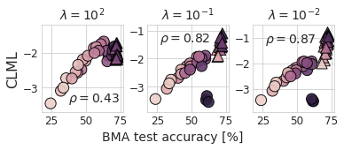
The paper shows that while the CLML is better correlated with the generalization performance of the model than the LML, the validation loss is still better correlated with the generalization performance than the CLML. Interestingly, the initially published DNN experiments in the first arXiv version of the paper did not actually compute the CLML but instead computed the validation loss. This was fixed in the second arXiv revision.This bug was found by yours truly, see the appendix of this post.

However, given the previous discussions on the similarities between the CLML and cross-validation and difficulty of approximating the CLML meaningfully, this bug was not a major issue for the paper’s conclusions.

Importantly, as we examine in the appendix of this post, when comparing the CLML using Monte Carlo sampling with the validation loss computed using Monte Carlo sampling for the Bayesian Model Average (BMA), the validation loss is still better correlated with the generalization performance than the CLML.

Conclusion

In conclusion, this blog post has challenged the conventional focus on the marginal likelihood and related quantities for Bayesian model selection as a direct consequence of Occam’s razor. It highlights the importance of considering context and goals when choosing a model selection criterion. By motivating MLE and MAP using Occam’s razor and questioning the uniqueness of the (conditional) joint marginal likelihood, we hope to encourage critical thinking about the foundations of these quantities.

However, it is important to acknowledge the limitations of our arguments and experiments. A more rigorous theoretical justification, a broader range of models and datasets, and a deeper engagement with philosophical implications are needed to strengthen the insights. As most of the presented methods ignore model complexity and assume a uniform model prior \(\pof{\h}\), we have not discussed it in the detail necessary, even though from the perspective of model description lengths (MDL), it would be crucial to take into account.

Despite these limitations, our exploration of the connections between information-theoretic concepts and their behavior in different data regimes, along the lines of model misspecification and prior-data conflict, provides a necessary starting point for understanding recently proposed metrics.

The toy experiment demonstrates that all discussed quantities can fail to reliably predict generalization under model misspecification and prior-data conflict, even for a basic setting using Bayesian linear regression. This emphasizes the need for caution when making claims about the superiority of any particular metric.

Ultimately, the key takeaway is that there is no one-size-fits-all solution, and the choice of model selection criterion should be guided by a careful consideration of the specific context and goals at hand.

Acknowledgements: We would like to thank the authors of the examined papers for their valuable contributions to the field and for inspiring this blog post, and to Freddie Bickford Smith for helpful comments and suggestions. Claude-3 and GPT-4 were used to edit and improve this blog post (via cursor.sh).

Reproducibility: The figures were created using matplotlib and seaborn in Python. The Bayesian linear regression model was implemented using numpy. The code for the toy experiment is available in this Google colab, and the code for the visualizations is available in this Google colab.

Appendix

Detailed Code Review of the DNN Experiments in Lotfi et al. (2022)

The logcml_ files in the repository contain the code to compute the CLML for partially trained models. However, instead of computing

the code computes:

which is the validation cross-entropy loss of the BMA (of the model trained with 80% of the training data).

The high-level code that computes the CLML is:

1
2
3
4
5
 
bma_accuracy, bma_probs, all_ys = get_bma_acc(
    net, la, trainloader_test, bma_nsamples, 
    hessian_structure, temp=best_temp
)
cmll = get_cmll(bma_probs, all_ys, eps=1e-4)
 

get_bma_acc marginalizes over the LA samples before returning bma_probs:

1
2
3
4
5
6
7
8
9
10
11
12
13
14
15
16
17
18
19
20
21
 
[...]
for sample_params in params:
    sample_probs = []
    all_ys = []
    with torch.no_grad():
        vector_to_parameters(sample_params, net.parameters())
        net.eval()
        for x, y in loader:
            logits = net(x.cuda()).detach().cpu()
            probs = torch.nn.functional.softmax(logits, dim=-1)
            sample_probs.append(probs.detach().cpu().numpy())
            all_ys.append(y.detach().cpu().numpy())
        sample_probs = np.concatenate(sample_probs, axis=0)
        all_ys = np.concatenate(all_ys, axis=0)
        all_probs.append(sample_probs)

all_probs = np.stack(all_probs)
bma_probs = np.mean(all_probs, 0)
bma_accuracy = (np.argmax(bma_probs, axis=-1) == all_ys).mean() * 100

return bma_accuracy, bma_probs, all_ys
 

The important line is #18: bma_probs = np.mean(all_probs, 0) which marginalizes over the predictions and returns the BMA prediction for each sample.

Finally, get_cmll computes the validation loss for each sample independently (after applying a bit of label smoothing):

1
2
3
4
5
6
7
8
9
10
11
 
def get_cmll(bma_probs, all_ys, eps=1e-4):
    log_lik = 0      
    eps = 1e-4
    for i, label in enumerate(all_ys):
        probs_i = bma_probs[i]
        probs_i += eps
        probs_i[np.argmax(probs_i)] -= eps * len(probs_i)
        log_lik += np.log(probs_i[label]).item()
    cmll = log_lik/len(all_ys)
    
    return cmll
 

The DNN experiments in Section 5 and Section 6 of the first arXiv revision of the paper (v1) thus did not estimate the CLML per-se but computed the BMA validation loss of a partially trained model (80%) and find that this correlates positively with the test accuracy and test log-likelihood of the fully trained model (at 100%). This is not surprising because it is well-known that the validation loss of a model trained 80% of the data correlates positively with the test accuracy (and generalization loss).

Author Response from 2022

The following response sadly seems to target the first draft mainly. However, it is also helpful for the final blog post and provides additional context.

Thanks for your interest in our paper and your comments. Here are our comments about the blog as it is currently framed:

(1) Thank you for pointing out a bug in the CLML computation for Figure 5b. We note that this bug is only relevant to a single panel of a single figure in the main text. We have re-run this experiment with the right CLML, and the results, attached here, are qualitatively the same. In summary, it was a very minor part of the paper, and even for that part it did not affect the take-away. We also attach the results of the correlation between the BMA test accuracy and the negative validation loss. You suggest in your post that the validation loss might correlate better with the BMA test accuracy than the CLML given that we use 20 samples for NAS. Our empirical results show the opposite conclusion. Additionally, we are not suggesting the CLML as a replacement to cross-validation but rather as a minor way to modify the LML for improvements in predicting generalization. Finally, we attach results for different sample sizes (20 samples vs. 100 samples) to address your comments on the sample size used to estimate the CLML. As we can see in the figure, the Spearman correlation factor is quite similar. 20 samples appears to provide a reasonable estimate of the CLML for these purposes, and is different from validation loss.

(2) Your post currently opens by suggesting that there is something wrong with our experiments, likely either an LML approximation or a CLML issue, because we note that the LML correlates more poorly with generalization for larger datasets (where “large” is relative in the context of a specific experiment). A few points here: (i) this result is actually completely expected. The LML is in fact non-monotonic in how well it predicts generalization. For small datasets, the prior should be reasonably predictive of generalization. For intermediate datasets, the first terms in the LML decomposition have a negative effect on the correlation with generalization. For asymptotically large datasets, the first terms have a diminishing effect, and we get a consistent estimator; (ii) almost all of our experiments are exact, and we see this behaviour in the exact experiments for the Fourier model. For example, for the Fourier feature experiment in Fig 4(d), LML picks the better generalizing model for n < 50 and n > 296. For n in [50, 296] it picks the wrong model. For large neural network models, it is reasonable that the exact LML could pick the wrong model for CIFAR-sized datasets. (iii) any potential issues with the CLML are not relevant to these considerations, which are about the behaviour of the LML.

(3) Your post currently suggests that issues with approximate inference could be responsible for our take-aways, rather than issues with the LML in general. But as we note in (2), almost all of our experiments use the exact LML and CLML: the density model, Fourier features, Gaussian processes, and deep learning exps on DKL, and there was never any bug associated with CLML computation in these experiments. The takeaways for the Laplace experiments are consistent with the exact experiments, and also expected, as above. While it’s true that the CLML can be estimated more effectively than the LML for the Laplace experiments, this is actually an advantage of the CLML that we note in the paper. The LML results also stand on their own, as we discuss above.

(4) Your post places a lot of importance on Figure 5, as if it is the main result of the paper and our main “DNN” experiments. We stand by the results of Figure 5, but it is a relatively minor component of the paper. As we’ve mentioned most of our results are exact, including our DKL experiments, which are certainly the most substantial DNN experiments, with practically exciting results for transfer and few-shot learning. The DKL experiments are actually where we expect the CLML to be practically useful, and currently they seem to be overlooked in the post.

(5) The blog seems to question the learning curve experiments, but these experiments in Figure 4 are exact, with no Laplace approximation, and relatively straightforward.

(6) Your post seems to be negative about the CLML, presenting its similarity with cross-validation as a potential drawback, and implying the skepticism about the CLML should affect the interpretation of our take-aways. Two points here: (i) as above, the CLML is independent of most of our take-aways, which are about the properties of the LML; (ii) our goal with the CLML was not to introduce something starkly different from cross-validation, but to show how a very minor modification to the LML could improve alignment with generalization. Moreover, the DKL CLML results are quite promising as an efficient way to do gradient based estimation of a large number of hyperparameters.

(7) The blog opens as if it is leading up to some fatal flaw. But as above, (i) the LML considerations are independent of the CLML, (ii) most of the experiments are exact, (iii) the trends for the exact and approximate inference procedures are the same and are naturally understandable and explainable, such as the non-monotonic trend in how well the LML correlates with generalization, and (iv) the CLML bug only affected Figure 5, panel b, and when it’s corrected the qualitative take-away is the same as before.

We appreciate your interest and effort in reading the paper, and we think your questions will improve the clarity of the paper, which we have updated with an acknowledgement to you. Given the above considerations, we do think there would need to be substantial revisions to the blog post to accurately and fairly reflect the paper. We would appreciate being able to see the revisions before it’s posted.

Best wishes,
Sanae, Pavel, Greg, Micah, Andrew

Ablation: CLML vs. BMA Validation Loss vs. (non-BMA) Validation Loss

Let us examine the new results:

In the three panels below, two panels show test accuracy vs. validation loss; one shows test accuracy vs. CLML. The left-most panel is the BMA test accuracy vs. (negative) BMA validation loss, the middle panel is vs. the CLML, and the right-most panel is vs. the (negative) non-BMA validation loss.

Note that the left-most panel is from v1, which was accidentally computing the BMA validation loss, and whose axis label is adapted here from v1 for clarity. The two other plots are from v2 after fixing the bug. See commits here for fixing the CLML estimation and here for computing the non-BMA validation loss.

At first glance, there might be an observer effect in the experiments for the validation loss. The BMA validation loss in v1 performs better than the CLML in v2, while the non-BMA validation loss in v2 underperforms the CLML in v2. When asked about it, the authors pushed the respective code (see link above) and explained that the updated, right-most panel computes the non-BMA validation loss, i.e., without LA samples. It seems surprising that there is such a difference between the non-BMA validation loss and BMA validation loss: the non-BMA validation loss is more than one nat worse on average than the BMA validation loss, based on visual inspection. Note that the plots here and in the paper compute the average CLML and average validation loss and are thus directly comparable.

The authors said in their response that:

You suggest in your post that the validation loss might correlate better with the BMA test accuracy than the CLML given that we use 20 samples for NAS. Our empirical results show the opposite conclusion.

This is only partially true. The BMA validation loss (which was accidentally computed in v1 instead of the CLML) correlates very well with the BMA test accuracy. This is not surprising given that this is the frequentist purpose of using validation sets. If validation sets were not correlating well with the test accuracy, we would not be using them in practice. 🤗 As such, this raises the question why the non-BMA validation loss correlates negatively with the BMA test accuracy for ResNets and overall in the v2 results. Thus, only the non-BMA validation loss supports the now opposite conclusion in v2 of the paper and in the authors’ response.

Yet what is also surprising is how well the BMA validation loss does vs. the CLML:

Ablation: LA Sample Size

Secondly, when we compare the reported values between BMA validation loss and CLML, we notice that the CLML is lower than the BMA validation loss by half a nat for \(\lambda=10^2\) and generally for CNNs.

However, it seems, even though the new experiments in v2 are supposed to reproduce the ones from v1, and we can assume that the same model checkpoints were used for re-evaluation (as retraining is not necessary), both CLML and non-BMA validation loss are off by about half a nat for the CNNs. As such, the above consideration might hold but might not provide the answer here.

Instead, we overlay the non-BMA validation loss and the CLML plots, both from v2, with a “difference blend”: it shows the absolute difference between the colors for overlapping data points (the circles 🔴 and triangles 🔺), leading to black where there is a match, negative (green-ish) color for CLML, and positive (sepia) color for validation losses. The background grids were used to match the plots, but we hid the ones from CLML afterward—as such, the strong overlay is because the values are so close.

Surprisingly—or rather as predicted when the LA does not really do much—it turns out that the validation loss for the CNNs (🔴) mostly fully matches the estimated CLML with 20 LA samples following a visual inspection. To be more precise, either the models have already sufficiently converged, or the CLML estimate is not actually capturing the correlations between points and thus ends up being very similar to the validation loss.

This changes the interpretation of the sample ablation in the author’s response. The ablation shows no difference between 20 and 100 LA samples, with 100 LA even samples having a slightly lower rank correlation. So it seems 5 times more LA samples are not sufficient to make a difference, or the Laplace posterior cannot capture the posterior as well as hoped. It would be interesting to examine this further. Kirsch et al (2022) reported running toy experiments on MNIST with 10,000 MC Dropout samples without achieving good adaptation. Laplace approximation is not MC Dropout, and this is speculation, but it seems in agreement. Notwithstanding the compute cost and feasibility, could posterior samples using HMC or similar more principled methods provide better estimates?

All in all, given the above, it is fair to say that the estimate of the CLML is probably not as good as hoped, and further experiments might be needed to tease out when the CLML provides more value than the (BMA) validation loss. Note, however, that this question has not been explicitly examined in the paper. Instead, for DNNs, the paper only compares LML and CLML with distinct estimation methods.