How to compute Hessian-vector products?

The product between the Hessian of a function and a vector, the Hessian-vector product (HVP), is a fundamental quantity to study the variation of a function. It is ubiquitous in traditional optimization and machine learning. However, the computation of HVPs is often considered prohibitive in the context of deep learning, driving practitioners to use proxy quantities to evaluate the loss geometry. Standard automatic differentiation theory predicts that the computational complexity of an HVP is of the same order of magnitude as the complexity of computing a gradient. The goal of this blog post is to provide a practical counterpart to this theoretical result, showing that modern automatic differentiation frameworks, JAX and PyTorch, allow for efficient computation of these HVPs in standard deep learning cost functions.

Hessian-vector products (HVPs) play a central role in the study and the use of the geometric property of the loss function of deep neural networks, as well as in many recent bilevel optimizers. However, computing such quantity is often considered prohibitive by practitioners, discouraging them from using algorithms that rely on HVPs.

With this blog post, we aim to convince the practitioners that with modern automatic differentiation (AD) frameworks such as JAX or PyTorch, HVPs can be efficiently evaluated. Indeed, standard AD theory predicts that the computational cost of an HVP is of the same order as the cost of computing a gradient. After a brief introduction on why HVPs are useful for optimization and ML applications and on the basis of AD, we explain in detail the AD-based methods to compute an HVP and the reason for their efficiency. In particular, we show that one can compute HVPs without explicit Hessian computation. We then compare the different methods to compute HVPs for several deep neural network architectures in terms of time and memory for both JAX and PyTorch. Our results illustrate the complexity predicted by the theory, showing that computing an HVP is not much more expensive than computing a gradient. This opens an avenue to develop efficient second-order informed methods for neural networks.

What are HVPs and where are they useful?

Let us first introduce the notion of Hessian and HVP. We will consider in this post a twice differentiable function \(f:\mathbb{R}^d\to\mathbb{R}\) that goes from a vector \(x\) in space \(\mathbb{R}^d\) to a real number in \(\mathbb{R}\). This typically corresponds to a function that maps the value of the parameters \(\theta\) of a neural network to the loss \(f(\theta)\). For such a function, standard AD can be used to efficiently compute the gradient of the loss \(\nabla f(\theta) = \left[ \frac{\partial f}{\partial \theta_i}(\theta)\right]_{1\le i \le d} \in \mathbb{R}^d\), using the backpropagation. The Hessian matrix of \(f\) at \(\theta\) is the matrix of its second-order partial derivatives

\[\nabla^2 f(\theta) = \left[\frac{\partial^2f}{\partial \theta_i\partial \theta_j}(\theta)\right]_{1\leq i,j\leq d}\in\mathbb{R}^{d\times d}\enspace.\]

This matrix corresponds to the derivative of the gradient and captures how the gradient will change when moving \(x\). To evaluate the variation of the gradient when moving \(\theta\) in the direction \(v\in\mathbb{R}^d\), one can compute the quantity \(\nabla^2 f(\theta) v\in\mathbb{R}^d\). This is the Hessian-vector product (HVP).

Let us review some use cases of HVPs in optimization and machine learning.

Inverse Hessian-vector products (iHVPs) in optimization

When trying to find the minimum of the function \(f\), methods that account for the second-order information often rely on the product between the inverse Hessian and a vector to find a good update direction. For instance, Newton’s method relies on update rules of the form

\[\theta_{k+1} = \theta_k - \eta_k[\nabla^2f(\theta_k)]^{-1}\nabla f(\theta_k)\]

for some step-size \(\eta_k>0\).

When evaluating the term \([\nabla^2f(\theta_k)]^{-1}\nabla f(\theta_k)\), it would be very inefficient to first compute the full Hessian matrix \(\nabla^2f(\theta_k)\), then invert it and finally multiply this with the gradient \(\nabla f(\theta_k)\). Instead, one computes the inverse Hessian-Vector Product (iHPV) by solving the following linear system

\begin{equation}\label{eq:linear_system} \nabla^2f(\theta)v = b\enspace. \end{equation}

with \(b = \nabla f(\theta_k)\). This approach is much more efficient as it avoids computing and storing the full Hessian matrix, and only computes the inverse of the matrix in the direction \(v\).

A second use case for the iHVP in optimization is with bilevel optimization. In bilevel optimization, one wants to solve the following problem

\begin{equation}\label{eq:bilevel_pb} \min_{x\in\mathbb{R}^d} h(x) = F(x, y^* (x))\quad\text{with}\quad y^*(x) = \arg\min_{y\in\mathbb{R}^p} G(x, y)\enspace. \end{equation}

The gradient of the function \(h\) can be computed using the implicit function theorem, giving the following expression

\[\nabla h(x) = \nabla_x F(x, y^* (x)) - \nabla_{xy}G(x, y^*(x))[\nabla_{yy}G(x, y^*(x))]^{-1}\nabla_y G(x, y^*(x))\enspace.\]

Here, the term \(\nabla^2_{yy} G(x, y)\) is the Hessian of the function \(G\) relatively to \(y\). Thus, this quantity also requires computing an iHVP.

To compute the iHVP, there are many methods in the literature to solve \eqref{eq:linear_system}, like Neumann iterates, the Conjugate Gradient method or gradient descent steps in the quadratic form \(v\mapsto \frac12\langle\nabla^2f(\theta)v, v\rangle - \langle b, v\rangle\). These methods rely on HVPs, as illustrated by the highlighted terms in the Conjugate Gradient method. Thus, an efficient implementation of HVPs is crucial for the overall algorithm performance.

Conjugate gradient to solve \eqref{eq:linear_system}
Input Initialization \(v_0\)
Initialization $$ r_0 = \textcolor{orange}{\nabla^2f(\theta) v_0} - b,\quad p_0 = -r_0,\quad t = 0 $$ While \(r_t \neq 0\) \begin{align*} \alpha_t &=\frac{r_t^\top r_t}{p_t^\top \textcolor{orange}{\nabla^2f(\theta) p_t}} \\ v_{t+1} &=v_t + \alpha_t p_t \\ r_{t+1} &=r_t + \alpha_t\textcolor{orange}{\nabla^2f(\theta) p_t} \\ \beta_{t+1} &=\frac{r_{t+1}^\top r_{t+1}}{r_t^\top r_t} \\ p_{t+1} &=-r_{t+1} + \beta_{t+1} p_t\\ t &=t + 1 \end{align*}

HVPs for the study of the loss landscape

The study of the geometry of neural networks is an active field that aims at understanding the links between training dynamics, local geometry of the training loss and generalization. One way to study the local geometry of a neural network is to find the distribution of the eigenvalues of its Hessian matrix. Indeed, depending on the sign of the eigenvalues of the Hessian, one can for instance distinguish local minima, local maxima and saddle points. As an illustration, the following figure shows how the sign of the eigenvalues of the Hessian matrix of a function affects the shape of the function’s landscape around a stationary point.

In several papers, an approximation of the Hessian spectrum is computed thanks to the Lanczos algorithm. This algorithm is a modification of the power method where each new iterate is taken in the orthogonal complement of the previous iterates. It outputs a factorization of the Hessian of the form $\nabla^2 f(\theta) = VTV^\top$ where \(V=(v_0,...,v_{k-1})\) is orthogonal and

\[T = \begin{pmatrix} \alpha_0& \beta_1 & 0 & \cdots & 0\\ \beta_1 & \alpha_1 & \beta_2 & \ddots & \vdots\\ 0 & \beta_2 & \alpha_2 & \ddots & 0\\ \vdots & \ddots & \ddots & \ddots & \beta_{k-1}\\ 0 & \cdots & 0 & \beta_{k-1} & \alpha_{k-1} \end{pmatrix}\enspace.\]

Lanczos' algorithm
Input Initial vector \(v_0\).
Initialization $$ w'_0 = \textcolor{orange}{\nabla^2f(\theta)v_0},\quad \alpha_0 = w_0'^\top v_0,\quad w_0 = w_0' - \alpha_0 v_0 $$ For \(i = 1,\dots, k-1\):
\begin{align*} \beta_i &= \|w_{i-1}\|\\ v_{i} &= \frac{w_{i-1}}{\beta_{i}}\\ w_i' &= \textcolor{orange}{\nabla^2f(\theta)v_i}\\ \alpha_i &= w_i'^\top v_i\\ w_i &= w_i' - \alpha_i v_i - \beta_iv_{i-1} \end{align*}

We observe once again that the Hessian information is accessed through HVPs rather than the full Hessian matrix itself.

A quick detour by automatic differentiation

Automatic differentiation (AD) is an important tool to compute exactly the derivatives of differentiable functions obtained as the composition of simple operations. There are two modes in AD; the forward mode that computes Jacobian-vector products (JVPs) and the reverse mode that computes vector-Jacobian products (VJPs). Since the gradient of a scalar function is a special case of the VJP, the reverse mode is the most frequently used in machine learning. It is typically used to compute the gradients of deep learning cost functions, where it is called backpropagation.

In what follows, we briefly present the notion of computational graph and the two AD modes. For a more detailed explanation, we refer the reader to the excellent survey by Baydin et al..

Computational graph

A key ingredient of AD is a computational graph associated with the code that evaluates a function. It is a directed acyclic graph that represents the succession of elementary operations required the evaluate a function.
Simple computational graph of a function \(f:\mathbb{R}^d\to\mathbb{R}^p\) are typically

In this graph, the vertices \(z_i\in\mathbb{R}^{m_i}\) represent the intermediate states of the evaluation of \(f\). To get the vertex \(z_i\), we use the values of its parents in the graph \(z_{i-1}\), with simple transfer functions \(z_i(z_{i-1})\). The computational complexity of the function evaluation depends on the complexity of the considered graph, as one node might have more than one parent. The memory footprint of the evaluation of the function is also linked to the maximum number of parents that can have a vertex in the computational graph, as their value needs to be stored until all children nodes have been computed.

Let us take an example with a multilayer linear perceptron (MLP) with 2 layers. The function \(f_x:\mathbb{R}^h\times \mathbb{R}^{h\times p}\to \mathbb{R}\) is defined for an input \(x\in\mathbb{R}^p\) by

\begin{equation}\label{eq:mlp} f_x(U, W) = \frac12(UWx)^2\enspace. \end{equation}

Here, the input \(\theta\) corresponds to the parameters of the network \((U, V)\) and the intermediate steps are \(z_1 = Wx\), \(z_2 = Uz_1\) and \(z_3 = \frac12 z_2^2\). A possible computational graph to get \(f_x(U, W)\) is the following

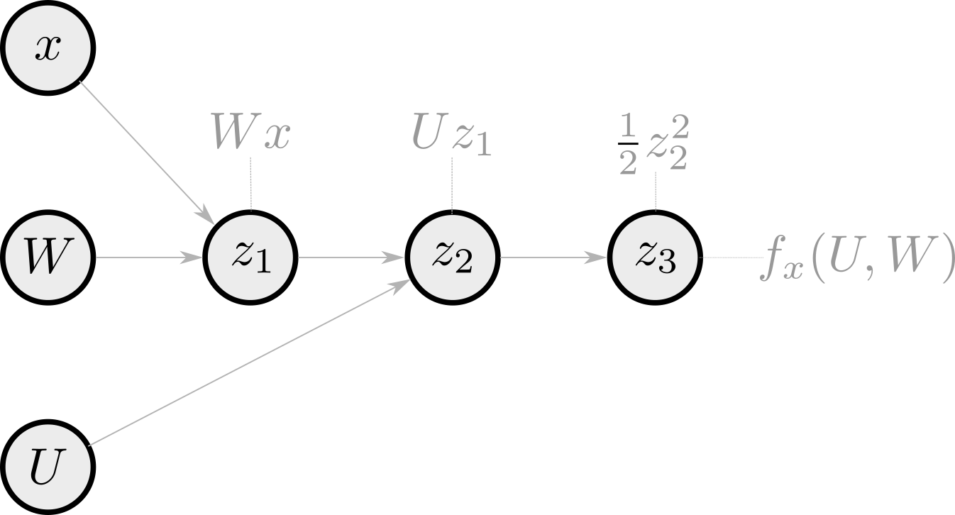
and the associated Python code to compute \(f_x\) is

def f(U, W):
    z1 = W @ x
    z2 = U @ z1
    z3 = 0.5 * z2**2
    return z3

Here, the feed-forward structure of the function makes the computational graph very simple, as each node has a single intermediate result parent.

AD uses this computational graph to compute the function’s derivatives. Using the chain rule, the Jacobian \(\frac{\partial f}{\partial \theta}(\theta)\) of \(f\) is obtained as a product of the Jacobian of the intermediate states \(z_1, \dots, z_n\). \begin{equation}\label{eq:chain_rule} \underbrace{\frac{\partial f}{\partial \theta}(\theta)}_{p\times d} = \frac{\partial z_n}{\partial \theta} =\frac{\partial z_n}{\partial z_1}\frac{\partial z_1}{\partial \theta}=\cdots = \underbrace{\frac{\partial z_n}{\partial z_{n-1}}}_{p\times m_{n-1}}\underbrace{\frac{\partial z_{n-1}}{\partial z_{n-2}}}_{m_{n-1}\times m_{n-2}}\cdots\underbrace{\frac{\partial z_1}{\partial \theta}}_{m_1\times d}\enspace. \end{equation} Depending on the order of the multiplication, one can compute the derivative of \(f\) with respect to \(\theta\) in two ways: the forward mode and the reverse mode.

Forward mode

For a vector $v\in\mathbb{R}^d$, the Jacobian-vector product (JVP) corresponds to the directional derative of $f$ in the direction $v$. It can be computed by the forward mode AD

\begin{equation}\label{eq:chain_rule_jvp} \frac{\partial f}{\partial \theta}(\theta)\times v = \frac{\partial z_n}{\partial z_{n-1}}\frac{\partial z_{n-1}}{\partial z_{n-2}}\cdots\frac{\partial z_1}{\partial \theta}v\enspace. \end{equation}

It consists in doing the multiplications in \eqref{eq:chain_rule_jvp} from the right to the left. It is a forward pass in the computational graph where we propagate at the same time the states \(z_i\) and the partial derivatives \(\frac{\partial z_{i+1}}{\partial z_i}\). If \(f\) is real-valued, the \(i\)th coordinate of its gradient is exactly given by product of the Jacobian of \(f\) and the \(i\)th canonical basis vector \(e_i\) since \begin{equation} \frac{\partial f}{\partial \theta_i}(\theta) = \lim_{t\to 0}\frac{f(\theta+te_i)-f(\theta)}{t}\enspace. \end{equation} Thus, we can get its gradient by computing each of the \(d\) JVPs \(\left(\frac{\partial f}{\partial \theta_i}(\theta)\times e_i\right)_{1\leq i \leq d}\) with forward AD.

To understand properly what is happening when using forward differentiation, let us go back to the linear MLP defined in \eqref{eq:mlp}. If we implement ourselves the forward differentiation to get the JVP, we obtain the following code

def jvp(U, W, v_u, v_w):
    # Forward diff of f
    z1 = W @ x
    v_z1 = v_w @ x  # Directional derivative of W -> W @ x in the direction v_w
  
    z2 = U @ z1
    v_z2 = U @ v_z1 + v_u @ z1  #  Directional derivative of (U, z_1) -> z2 in the direction (v_u, v_z1)
  
    v_z3 = v_z2 @ z2  # Directional derivative of z2 -> .5*z2**2 in the direction v_z2 
    return v_z3

In comparison with the code of the evaluation of \(f_x\), there are two more operations corresponding to the computation of the dual variables v_z1 and v_z2. In terms of memory, if we consider the computation of the JVP as coded in the previous snippet, the maximum number of parents of a vertex is four. This maximum is achieved by the vertex v_z2 which has the vertices U, v_z1, v_u and z1 as parents.

In JAX, we get the JVP of a function \(f\) in the direction \(v\) with jax.jvp(f, (params, ), (v, ))[1].

Reverse mode

The reverse mode is also known as backpropagation in the context of deep learing. For $u\in\mathbb{R}^p$, it aims at computing VJPs

\begin{equation}\label{eq:chain_rule_vjp} u^\top\frac{\partial f}{\partial \theta}(\theta) = u^\top\frac{\partial z_n}{\partial z_{n-1}}\frac{\partial z_{n-1}}{\partial z_{n-2}}\cdots\frac{\partial z_1}{\partial \theta}\enspace. \end{equation}

In the reverse AD, the multiplications of \eqref{eq:chain_rule_jvp} are done from the left to the right. It requires doing one forward pass in the computational graph to compute the intermediate states \(z_i\) and then a backward pass to propagate the successive partial derivatives from the left to the right. Contrary to the forward mode, it has a more important memory footprint. Indeed, it requires storing the values of all the states. For instance, to compute the last term \(\frac{\partial z_3}{\partial z_2}\), one needs the value of \(z_2\) which was the first computed during the forward pass. If \(f\) is real-valued, \(u\) is a scalar and the VJP is the multiplication of the gradient of \(f\) by \(u\). Thus, one can get the gradient on \(f\) by using \(u=1\) and performing only one reverse differentiation. This makes this mode more efficient in computing gradients.

Let us observe what happens if we code manually the backpropagation to get the gradient of the previous function \(f_x\) defined by \(f_x(U, W) = \frac12(UW x)^2\).

def gradient(U, W):
    # Forward pass
    z1 = W @ x
    z2 = U @ z1
    z3 = 0.5 * z2**2

    # Reverse pass
    ## Transfer function: z3 = 0.5 * z2**2
    dz2 = z2  # derivative of z3 wrt z2
  
    ## Transfer function: z2 = U @ z1
    dU = jnp.outer(dz2, z1)  # derivative of z3 wrt U
    dz1 = U.T @ dz2  # derivative of z3 wrt z1
  
    ## Transfer function: z1 = W @ x
    dW = jnp.outer(dz1, x)   # derivative of z3 wrt W
    
    return dU, dW

This function returns the gradient of \(f_x\). At reading this code, we understand one needs to store all the intermediate values of the forward pass in the graph. Indeed, if we look at the case of z1 which is the first node computed, it is used four steps later for the computation of dU.

To get the gradient in JAX, one can use jax.grad(f)(params).

Naive computation of HVPs

Since we are interested in computing \(\nabla^2 f(\theta)v\), the simplest way to do it is to compute the Hessian matrix and then multiply it by the vector \(v\). This can be achieved in JAX by calling jax.hessian(f)(params) @ v.

This method is quite cumbersome making it impossible to use for deep neural networks. Indeed, the storage of the full Hessian matrix has \(\mathcal{O}(d^2)\) complexity where \(d\) is the dimension of the model’s parameters set.

The good news is that we can compute HVP without computing the Hessian thanks to clever use of AD.

HVPs without explicit Hessian computation

In 1994, Pearlmutter proposed to leverage the following observation to compute HVP efficiently: the HVP is also the directional derivative of the gradient in the direction \(v\):

\[\nabla^2f(\theta) v = \lim_{\epsilon\to 0} \frac1\epsilon[\nabla f(\theta+\epsilon v)-\nabla f(\theta)] = \nabla [\langle \nabla f(.), v\rangle](\theta)\enspace.\]

Based on this identity, AD enables to compute HVPs in three ways, as described in the JAX documentation.

Forward-over-reverse

The forward-over-reverse mode consists in doing forward differentiation in a computational graph of the gradient of \(f\).

Its implementation in JAX is only two lines of code.

def hvp_forward_over_reverse(f, params, v):
  return jax.jvp(jax.grad(f), (params, ), (v, ))[1]

In this case, jax.grad(f)(params) is computed by backward AD, whose complexity is two times the complexity of evaluating \(f\). Thus, the temporal complexity of hvp_forward_over_reverse is roughly four times the complexity of the evaluation of \(f\).

To better see what happens, let us consider again our function \(f_x\) defined by \eqref{eq:mlp}. The Python code of the forward-over-reverse HVP is the following.

def forward_over_reverse(U, W, v_U, v_W):
    # Forward through the forward pass through f
    z1 = W @ x
    v_z1 = v_W @ x
  
    z2 = U @ z1
    v_z2 = U @ v_z1 + v_U @ z1
    
    # z3 = 0.5 * z2**2
    # Forward through the backward pass through f
    z4 = z2  # dz2
    v_z4 = v_z2  # v_dz2
  
    z5 = jnp.outer(z4, z1)  # dU
    v_z5 = jnp.outer(v_z4, z1) + jnp.outer(z4, v_z1)  # v_dU
  
    z6 = U.T @ z4  # dz1
    v_z6 = U.T @ v_z4 + v_U.T @ z4  # v_dz1
  
    z7 = jnp.outer(z6, x)  # dW
    v_z7 = jnp.outer(v_z6, x)  # v_dW
  
    return v_z5, v_z7  # v_dU, v_dW

The take-home message of this part is that, after computing the gradient of \(f_x\), one can consider a computational graph of this gradient and perform forward differentiation through this new computational graph. Here, the variables z1,…, z7 are the vertices of a computational graph of the gradient of \(f_x\). The nice thing is that this mode enables getting at the same time the gradient and the HVP. Indeed, in the previous snippet, z5 and z7 are the components of the gradient of \(f_x\) which could be also returned if needed. This feature can be useful in bilevel optimization for instance.

Reverse-over-reverse

Instead of doing forward differentiation of the gradient, one can multiply the gradient by \(v\) and thus get a scalar. We can then backpropagate into this scalar product. This is the reverse-over-reverse mode.

It can be implemented by these lines of code.

def hvp_reverse_over_reverse(f, params, v):
  return jax.grad(lambda y: jnp.vdot(jax.grad(f)(y), v))(params)

Since the gradients are computed by backpropagation, the complexity of hvp_reverse_over_reverse is twice the complexity of jax.grad(f), which is roughly four times the complexity of the evaluation of \(f\).

Writting down the code of the reverse-over-reverse HVP for our function \(f_x\) defined by \eqref{eq:mlp} makes us understand the differences between this mode and the forward-over-reverse mode. Particularly, one can notice that there are more elementary operations in the reverse-over-reverse mode than in the forward-over-reverse mode. Moreover, in terms of memory footprint, the reverse-over-reverse requires storing the values of the vertices of the computational graph of the gradient of \(f_x\), while the forward-over-reverse only needs to store the values of the vertices of the computational graph of \(f_x\). Thus, the former is less efficient than the latter.

def reverse_over_reverse(U, W, v_u, v_w):
    # Forward through <grad(f), v>
    ## Forward through f
    z1 = W @ x
    z2 = U @ z1
    z3 = 0.5 * jnp.linalg.norm(z2)**2
  
    ## Reverse through f
    z4 = z2  # dz2
    z4 = jnp.outer(z3, z1) # dU
    z5 = U.T @ z3 # dz1
    z6 = jnp.outer(z5, x) # dW
  
    # Output: dot product <grad(f), v>
    z7 = jnp.sum(z4 * v_u) + jnp.sum(z6 * v_w)
  
    # Backward through z7 = <grad(f),v>
    ## z7 = jnp.sum(z4 * v_u) + jnp.sum(z6 * v_w)
    dz6 = v_w
    dz4 = v_u
  
    ## z6 = jnp.outer(z5, x)
    dz5 = dz6 @ x
  
    ## z5 = U.T @ z3
    dz3 = U @ dz5
    ddU = jnp.outer(z3, dz5)  # Derivative of z7 wrt U
  
    ## z4 = jnp.outer(z3, z1)
    dz3 += dz4 @ z1
    dz1 = dz4.T @ z3
  
    ## z3 = z2
    dz2 = dz3
  
    ## z2 = U @ z1
    dz1 += dz2 * U
    # As U appears multiple times in the graph, we sum its contributions
    ddU += jnp.outer(dz2, z1) 
  
    ## z1 = W @ x
    ddW = jnp.outer(dz1, x)  # Derivative of z7 wrt W
  
    return ddU, ddW

Reverse-over-forward

What about doing forward differentiation of \(f\) rather than reverse propagation? This is what is done in the reverse-over-forward mode. It consists in backpropagating in the computational graph of the JVP of \(f\) and \(v\).

def hvp_reverse_over_forward(f, params, v):
  jvp_fun = lambda params: jax.jvp(f, (params, ), (v, ))[1]
  return jax.grad(jvp_fun)(params)

This method is more efficient than the previous one. Indeed, since we backpropagate only once, the memory burden is lower than for the reverse_over_reverse fashion. In comparison with forward-over-reverse, the complexity is the same. However, one can notice that the forward-over-reverse enables computing at the same time the gradient of \(f\) and the HVP, which is not the case for the reverse-over-forward mode.

The code of the reverse-over-forward HVP for the MLP \(f_x\) defined by \eqref{eq:mlp} is the following.

def reverse_over_forward(U, W, v_U, v_W):
    # Forward diff of f to  <grad(f), v>
    z1 = W @ x
    z6 = v_W @ x  # v_z1
  
    z2 = U @ z1
    z5 = U @ z6 + v_U @ z1  # v_z2
  
    # output <grad(f), v>
    z4 = z5 @ z2  # v_z3
  
    # Backward pass through <grad(f), v>
    ## z4 = z5 @ z2
    dz2 = z5
    dz5 = z2  # dv_z2
  
    ## z5 = U @ z6 + v_U @ z1
    dz1 = v_U.T @ dz5
    dz6 = U.T @ dz5  # dv_z1
    ddU = jnp.outer(dz5, z6)  # derivative of z4 wrt U
  
    ## z2 = U @ z1
    # As U and dz1 appear multiple times, we sum their contributions
    dz1 += U.T @ dz2
    ddU += jnp.outer(dz2, z1)
    
    ## z1 = W @ x
    ddW = jnp.outer(dz1, x)
    return ddU, ddW

Benchmark with deep learning architectures

While these three methods compute the same outputs, the different ways of traversing the computational graph change their overall time and memory complexities. We now compare the computation of HVPs with these three methods for various deep-learning architectures. To cover a broad range of use cases, we consider a residual network (ResNet34) and a transformer-based architecture (ViT-base) for image classification as well as a transformer for natural language processing (Bert-base.). We use the Flax and PyTorch implementations of these architectures available in the transformers package provided by Hugging Face 🤗.

All computations were run on an Nvidia A100 GPU with 40 GB of memory. We used the version 0.4.21. of Jax and the version 2.1.1. of torch.

The code of the benchmark is available on this repo.

Time complexity

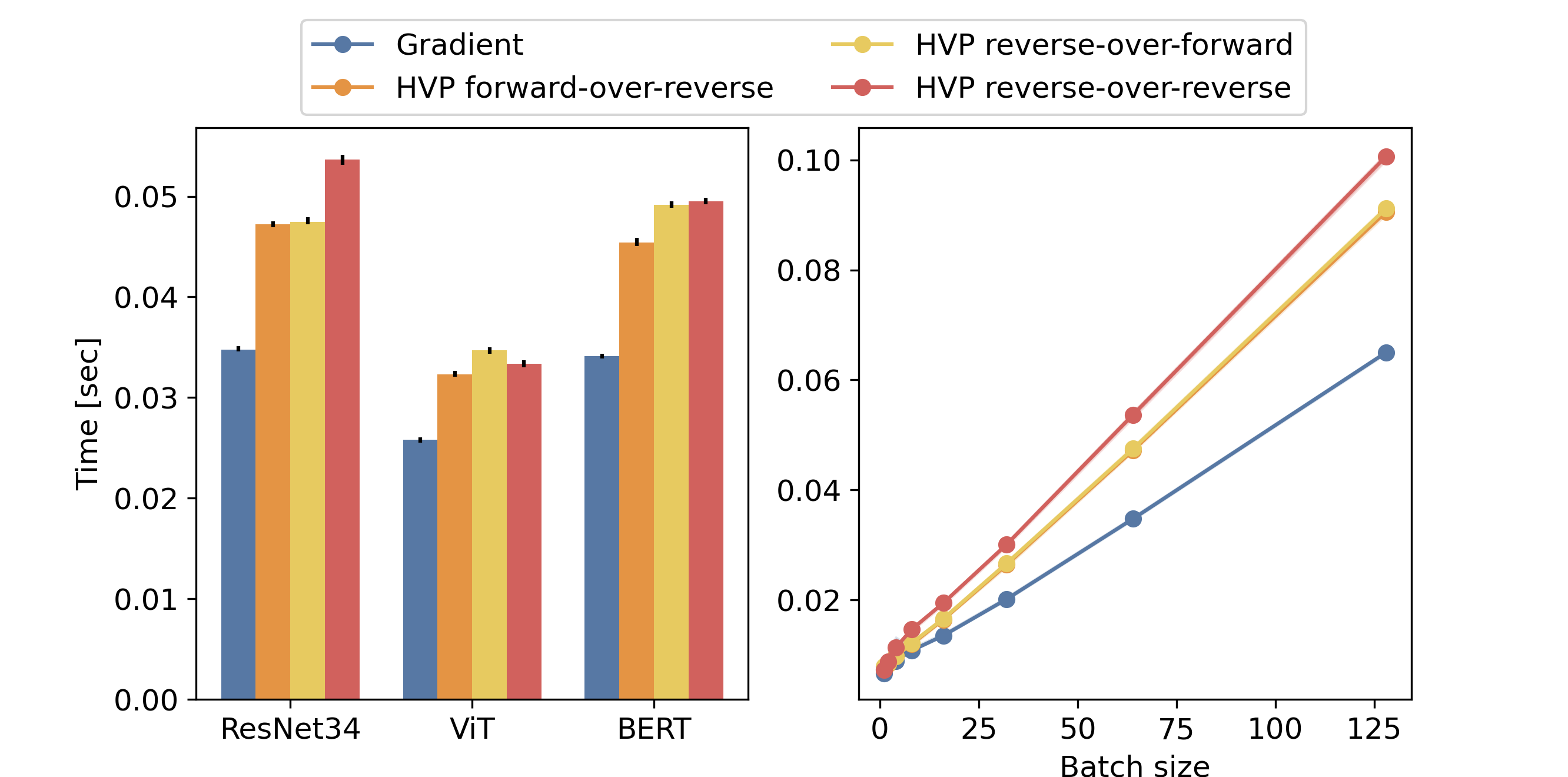
The first comparison we make is a comparison in terms of wall-clock time between the different ways to compute HVPs and also the computation of a gradient by backpropagation. For each architecture, we compute the gradient of the model with respect to the parameters by backpropagation. We also compute the HVPs in forward-over-reverse, reverse-over-forward and reverse-over-reverse modes. For each computation, we measure the time taken. Specifically for the HVPs, we subtract the time taken by a gradient computation, to get only the time of the overhead required by the HVP computation. The inputs for each architecture are generated randomly. For the ResNet34 architecture, we generated a batch of images of size 224x224x3. To limit out-of-memory issues in the experiments, we generated for the ViT architecture images of size 96x96x3. For the BERT architecture, we generated a batch of sequences of length 32.

We first use JAX with just-in-time compilation. Each computation is run 90 times. We plot on the left of the figure, the median computation time and also the 20% and 80% percentile in black. The computations are done with a batch size of 128. We observe that, in practice, the overhead over the gradient computation for the HVP computation is between one and twice the time of a gradient computation for the three architectures. Consequently, a whole HVP computation takes between twice and three times the time of a gradient calculation. This is consistent with the theory. One can notice that the reverse-over-reverse is slightly slower than the others in all the cases. The forward-over-reverse and reverse-over-forward are, as for them, very close in terms of time.

We also report on the right figure the computational time of each method with respect to the batch size for the ResNet34 architecture. We observe, as expected, that the computational time scales linearly with the batch size.

We run a similar experiment with the functional API available in PyTorch torch.func similar to the one JAX has. The results we get are more contrasted.

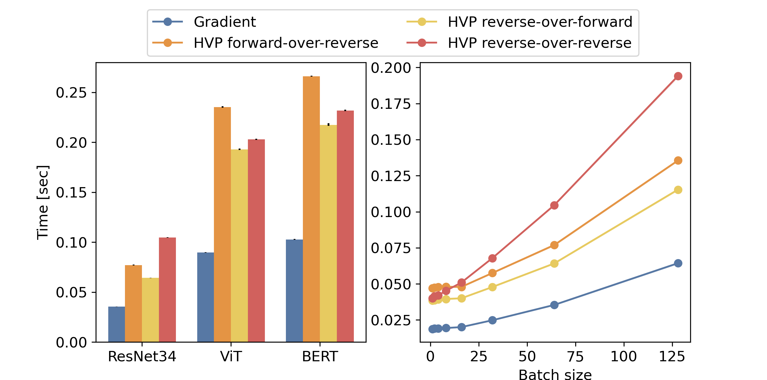
In the case of ResNet34, the scaling between the different methods is similar to the one we get with JAX. Also, during our experiments, we figured out that batch normalization made the forward computation slow and induced out-of-memory issues. Thus, we removed the batch normalization layers from the ResNet34 architecture.

For ViT and BERT, the forward-over-reverse is surprisingly longer than the reverse-over-reverse method. Moreover, the scaling between the gradient and HVP computational time differs from the one we get with JAX. Indeed, for these architectures, the HVP computations take between four and five more time than the gradient computations. This is a discrepancy with what we would expect in theory. This might be because, at the time we are writing this blog post, the functional API of PyTorch is still in its early stages. Particularly, we could not use the compilation with torch.compile because it does not work with some operators of torch.func such as torch.func.jvp.

Memory complexity

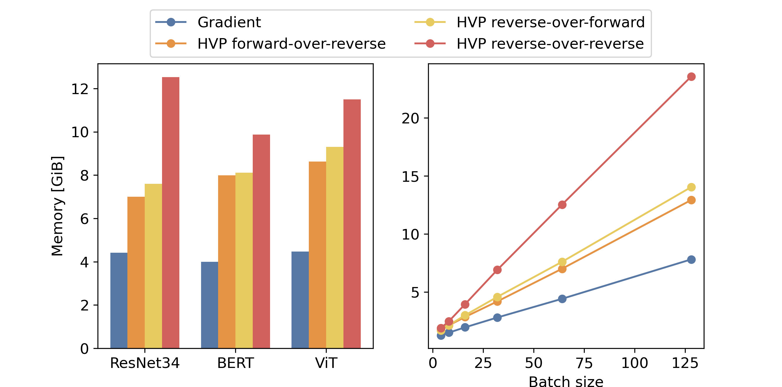
We also compare the memory footprint of each approach. The following figure provides the results we get with jax jitted code. On the left, we represent the result for each method and model with a batch size of 64. On the right, we show the evolution of the memory footprint of each method for the ResNet34 with the batch size. Surprisingly, we could observe that the memory footprint of the different methods to compute HVPs does not vary for a given model. This is counterintuitive since we expect that the reverse-over-reverse method have a larger memory footprint due to the double backpropagation.

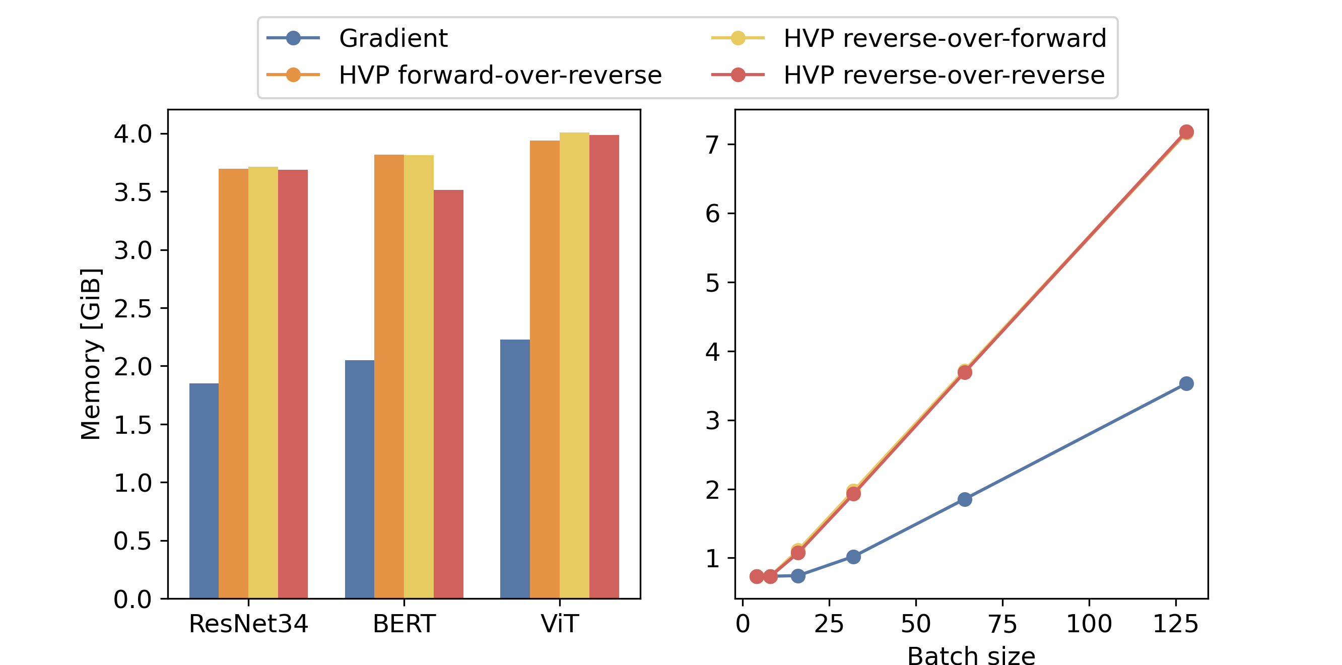
However, we do the same experiment by disabling the JIT compilation. The result we get corroborates the theory. Indeed, one can observe in the following figure that the memory footprint of the reverse-over-reverse method is larger than the one of the forward-over-reverse and reverse-over-forward methods. This is because the reverse-over-reverse involves two successive backward differentiations while the other two involve only one reverse differentiation. Moreover, it scales linearly with the batch size, which was not the case in the previous figure in the small batch size regime.

In light of these two results, the clever memory allocation performed during just-in-time compilation reduces significantly the memory footprint of the HVP computations.

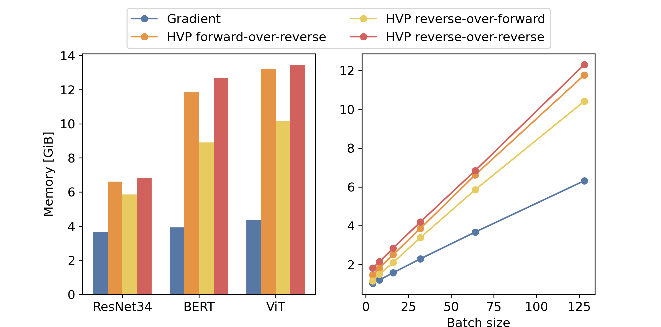
In the following figure, we plot the results we get with the PyTorch implementation. One can observe that in all the cases the forward-over-reverse consumes more memory in comparison with the reverse-over-forward mode. It is almost at the same level as reverse-over-reverse mode, which is quite unexpected.

The right plot of the evolution of the memory footprint with the batch size for the ResNet34 architecture evolves linearly as expected.

Conclusion

In this blog post, we have explored the different ways to compute HVP from theoretical and practical perspectives. The three take-home messages to keep in mind are the following:

• We can compute HVPs without computing Hessian matrices.

• In practice, computing an HVP takes between twice and four times the time taken by a gradient computation and requires two to three times more memory than computing a gradient.

• The AD framework and the use or not of the just-in-time compilation affects the practical performances of HVPs computations in time and memory.